An article in the author’s Astronomy Digest – http://www.ianmorison.com
This essay is a further example of imaging with a tracking mount as described in Chapter 3 of ‘The Art of Astrophotography’ and will also show how the free program IRIS can stretch images using the full 16-bits per colour output from Deep Sky Stacker before using the current 8-bit version of GIMP (also free) to complete the image processing.
In our northern skies we have two beautiful regions – one including the Orion, Taurus and Gemini constellations and the second the constellations Cygnus, Lyra, Delphinus and Aquarius. The southern skies have one region of equal beauty; that of the constellations Centaurus, Crux and Carina which lie along the plane of the Milky Way. I have long wanted to image this region and a trip to South Island, New Zealand in February this year (2017) gave an opportunity to do so. The constellations were visible for most of the short night and lay overhead in the hour before dawn.
Central South Island between Christchurch and Queenstown includes the Aoraki Mackenzie Dark Sky Reserve − one of only three ‘Gold Tier’ reserves in the world − and I spent a week in this region which, happily, included three nights which were clear for part of the time. The Moon was waxing and the imaging periods had to become later to avoid moonlight as the Moon, reaching first quarter, remained longer in the sky. It was a pity that my two nights within the dark sky reserve itself were not clear, though I have been able to image the centre of the Milky Way from there in the past.
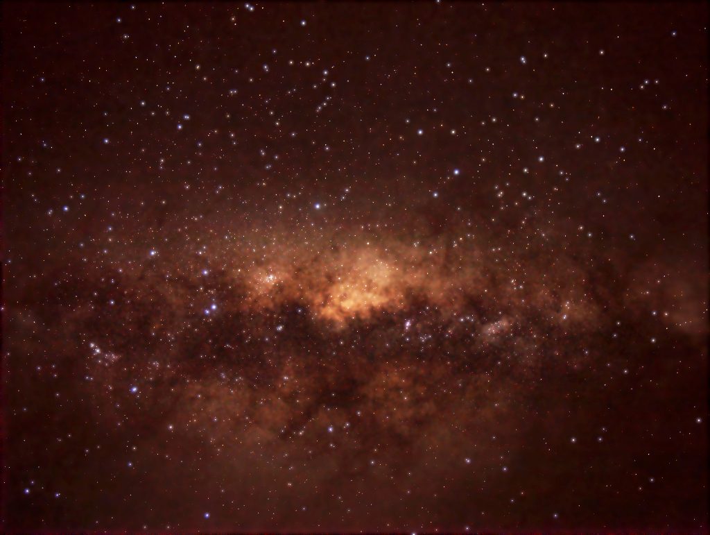
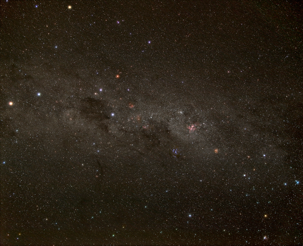
The centre of the Milky Way imaged from the Mt John Observatory, South Island, New Zealand.
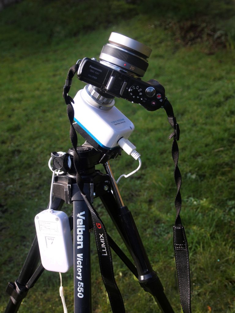
I had taken to New Zealand what is almost certainly the smallest and lightest imaging system that could be assembled. It was based on a Panasonic GX1 Micro 4/3, 16 megapixel, camera equipped with the superb Panasonic 20mm, f/1.7, prime lens of compact and lightweight ‘pancake’ design. To mount the camera I had brought with me a ‘Nano Tracker’ – the smallest tracking mount available − and a small ball and socket head. This is often called the Baader Nano Tracker but is, in fact, made by Sightron in Japan. These were all in my carry on luggage with a lightweight Velbon tripod having a ‘pan and tilt’ head in my checked-in case. The pan and tilt head is ideal for adjusting the azimuth and elevation of a tracking mount. The Nano Tracker only provides a small ‘sighting hole’ for polar alignment which is not very practical and, for use in the northern hemisphere, I have made an aluminium panel that sits between the tripod head and tracker and has a mounting aperture on one side for a laser pointer. Aligning on the South Celestial Pole (SCP) is not that easy and I simply used a compass to find south and its ‘ring’ as a protractor to set the elevation. The constellations I were imaging are not that far from SCP and so with exposures of just 60 seconds the alignment did not have to be too precise but, perhaps by chance, the alignment on my first imaging session was spot on.
The ‘long exposure noise reduction’ was, and should be, turned off. If employed, it takes a ‘dark frame’ with the same exposure as the light frame and then subtracts the two – which means, of course, that one is only imaging the sky for half the time. This process will remove ‘hot pixels’ and will also remove some amplifier glow that can be usually be seen along one edge of the frame. This is good but what is less well known is that subtracting a single dark frame will actually increase the noise in the image by ~41% as the dark frame is itself noisy. However when processing the images in Deep Sky Stacker one part of the process (if activated) aims to find and subtract off hot pixels. It may though be necessary to crop the final image a little to remove the part affected by amplifier glow. In the case of this image, the small area along one side showing amp glow (an excess of red) was selected and the levels tool applied to red was used to reduce its brightness. I did not want to crop the image as it included a nice open cluster. In my view it is far better to spend the whole imaging period imaging the sky. If, say, one had one hour of imaging 60 second sub-frames (usually called subs) then, if the noise reduction is turned off, twice as many subs will be stacked and the noise will be reduced by a factor of the square root of two or 1.414. If, however, the noise reduction is employed, the noise in the final image will be increased by ~0.4 making a difference of ~1.8 in relative noise performance.
At the end of the imaging session it could be worth covering up the lens and taking 10-20 dark frames to import into Deep Sky Stacker along with the light frames. These will then be taken with the sensor at approximately the same temperature as when the light frames were taken which is important − do not take them first. As explained in the chapter in ‘The Art of Astrophotography’ on cooling a DSLR, during the taking of continuous light frames the sensor will warm up by perhaps 12 degrees Celsius and if dark frames are to be used it would be sensible to take ‘dummy’ images continuously for ~15 minutes before taking the sub-frames that will be stacked along with the dark frames. I think that you can see that the use of dark frames when using a digital camera without set-point cooling is really rather tricky. The comparison below is of a single dark fame and the ‘master dark’ produced from stacking 24 dark frames. Both have been identically stretched.
![]()
Single and stack of 24 dark frames
Many modern digital cameras allow the hot pixels in their sensors to be mapped out by replacing the pixel with an average of the surrounding ones. This process is usually rather deep in the camera’s menus but, for example, in the case of the Panasonic GX1 used to take this image it is called ‘Pixel Refresh’. Having employed this process, no obvious hot pixels could be seen in the images.
There is a case for taking ‘flat frames’ or ‘flats’ if the lens that is to be used suffers from obvious vignetting towards the corners of the frame. Stopping the lens down by one or two stops will usually reduce the vignetting as well as improving the image quality away from the frame centre. To achieve both these aims, I had stopped the f/1.7 lens used to take this image down to f/2.5. Using this lens at f/2.5 the extreme corners will be less bright by ~half a stop. Flat frames are taken by using the same lens stop as when the light frames were taken whilst simply imaging a uniformly illuminated flat surface so that the peak brightness in the images are ~70% of maximum. A nice feature of the use of flat frames is that they will mitigate the effects of dust on the sensor. Putting a set of flats into DSS will even the brightness across the frame – but the outer parts will be somewhat noisier dependant on how much gain was required to bring up these areas.
Flat frames were taken by laying the camera on its back pointing up towards a diffuse inset roof light with a piece of A4 white paper held a few inches above the camera lens which was still focussed on infinity. This latter point is very important as the image scale changes as the focus is adjusted. These were imported into DSS along with the 21 light frames. The effect on the image using the flats was not that great (it is a good lens) but it did help to bring out an open cluster, C 96, near to the lower right of the image below the ‘False Cross’ in Carina.
I took 60 second exposures using an ISO of 800. Why did I choose this value? The fundamental point is that the data collected by the sensor is not altered as the ISO is changed. As the ISO is increased up to some value, the gain of the amplifiers reading out the data from the sensor is increased to make the sensor appear more sensitive. (This does increase the noise somewhat.) Above this ISO value, which differs from camera to camera, the values read out with the maximum amplifier gain are simply multiplied by factors of two increasing through 2,4,8 … as the ISO is increased. (This is bound to increase the perceived noise.) There is nothing gained in final image quality by going beyond the ISO value having maximum amplifier gain. This is around ISO 800 for many cameras and so this is the ISO I use. It can be worth using a far higher ISO initially so that the stars can be easily seen to frame the image but, for this image, I could make out the brightest stars in the field at ISO 800. [There is good case for using a camera with a swing-out live screen as, with the camera pointing near vertical, I was lying on my back to see the screen in order to frame the image! If the camera has a swing-out screen the thermal path from the sensor to the outside will be shorter and so the sensor should not increase in temperature so much as continuous exposures are made.]
Each exposure was initiated manually with a delay of 2 seconds to eliminate any vibrations. Both raw and Jpeg files were captured. The Jpegs make it very easy to scan though the images to find the start and end of the usable frames as, initially, some were used to set the framing.
The sky on my first imaging session from a relatively dark location between Arrowtown and Queenstown was partially cloudy with low level cloud passing rapidly across the sky. This may have been a good thing as I suspect that it ‘trapped’ much of the light pollution so giving a darker sky. Several of the frames would thus have been partially cloud covered so, rather than remove those frames from the stack I used the ‘median’ stacking mode with eliminates pixels whose brightness is significantly away from the mean. DSS was able to stack 19 out of the 22 frames that I had taken and, pleasingly, the effects of any clouds had been eliminated. My imaging session had to end as the cloud cover increased too much.
Processing the raw files
The current version of DSS (as of February 2017) cannot accept the .RW2 files produced by the Panasonic GX1 camera. However, the free Adobe program ‘Adobe DNG converter’ will accept them and convert the files into .dng format which DSS will accept. So these were stacked in DSS and the result saved as a Tiff file.
Stretching the Image
The next step is to ‘stretch’ the image to bring up its fainter parts. This really needs to be done using a 16-bit image depth and this can be achieved by employing the free program IRIS. The Tiff output file from DSS is simply loaded into IRIS (a completely white screen appeared!) and within the ‘View’ drop down menu ‘Logarithm’ clicked upon. This made three passes and then a very nicely stretched image appeared which was exported as an 8-bit bitmap file (.bmp). Thus stretching had been achieved with a 16-bit image depth.
Final Processing in GIMP
I had taken a lightweight notebook without my usual Photoshop software but was able to download GIMP 2.8. This version can only handle 8-bit depth for each colour. (The next formal (2.10) version will, I believe, be able to handle 16-bit images.) The IRIS .bmp file was imported into GIMP and a small further stretch was made by using the ‘Levels’ command in the ‘Colour’ drop down menu and sliding the middle slider a little to the left.
As I point out in the CUP books, digital images do not appear as good as those that used to be taken with film. Halation within the emulsion scatters the light of bright stars and increases their size in the image. As is used in sky charts, this makes them stand out better. I was able to image the region again and was a little surprised to find that the brighter stars were more prominent. I believe that the atmosphere was somewhat hazy and so scattered their light so I decided to use some of the data from the ‘hazy’ image to add its bright stars into the Arrowtown image. To produce an image showing just the bright stars the levels command was used to remove the fainter stars and a black paintbrush was used to remove some remaining regions of the Milky Way. The star’s colours were then enhanced somewhat using the ‘hue/saturation’ tool.
The brighter stars from a second imaging session where a hazy sky had increased their size
The initial image and the bright stars image were loaded as layers and the ‘Screen’ Blending mode set in the layers mode menu. With the bright stars layer selected, the ‘rotate image’ (in the layers drop down menu) and ‘move’ tools were used to align the bright stars image over those in the initial image. [This is much easier in Photoshop!] The two layers were then flattened (still using the ‘Screen’ blending mode) to give the final result shown below.
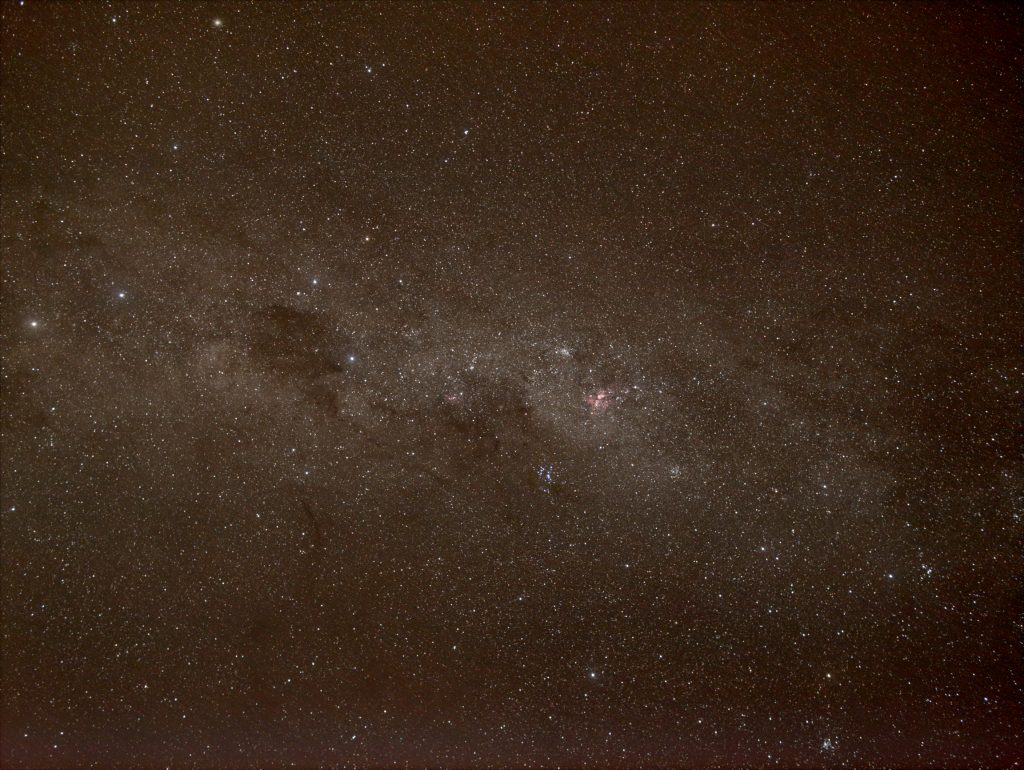
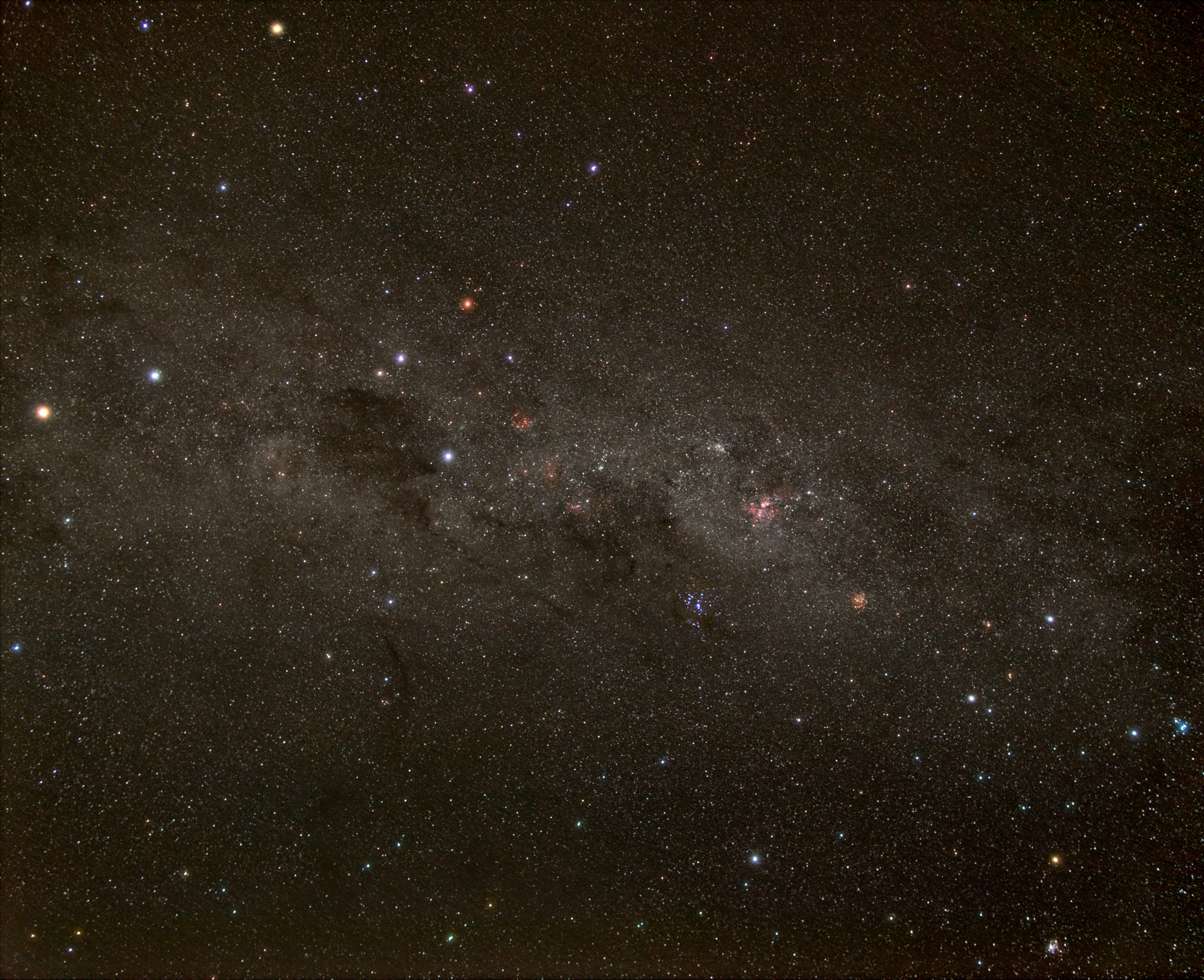
The image of the Southern Cross region with the enhanced brighter stars. A larger scale image can be found on the Jodrell Bank Night Sky website for March 2017 : http://www.jb.man.ac.uk/astronomy/nightsky/Southerncross.jpg
To the extreme centre left is Alpha Centauri (abbreviated Alpha Cen or α Cen) which is the closest star system to the Solar System at a distance of 4.37 light-years. It consists of three stars: the pair Alpha Centauri A (also named Rigil Kentaurus) and Alpha Centauri B together with a small and faint red dwarf star, Alpha Centauri C (named Proxima Centauri), that may be gravitationally bound to the other two and is, as its name suggests, the closest star to our Sun at a distance of 4.24 light years. To the unaided eye, the two main components appear as a single point of light with an apparent visual magnitude of −0.27, forming the brightest star in the southern constellation of Centaurus and the third-brightest star in the night sky, outshone only by Sirius and Canopus.
In complete contrast, Beta Centauri or Hadar, is a triple star system that lies at a distance of ~390 light years so must be fundamentally very bright indeed. The combined system is 41,700 times brighter than our Sun and so is one of the brightest star systems that can be seen with our unaided eyes. Moving up to the top of the image at ~45 degrees from Beta Centauri is Omega Centauri: long thought to be a globular cluster, it is now suspected to be the core of a galaxy whose outer stars have been stripped off by the gravitational effects of the Milky Way. It may even have a ‘black hole’ at its heart. Alpha and Beta Centauri act as ‘the pointers’ towards the Southern Cross or Crux that lies to the upper right of the dark dust region called the Coalsack. Just below the left hand star of Crux lies a very tight open cluster called the ‘Jewel Box’. John Herschel said of it: “this cluster, though neither a large nor a rich one, is yet an extremely brilliant and beautiful object when viewed through an instrument of sufficient aperture to show distinctly the very different colour of its constituent stars, which give it the effect of a superb piece of fancy jewellery”.
Further along the Milky Way is a pinkish region (due to H-alpha emission) called the Eta Carina Nebula. At its heart is the star Eta Carina which is in the final stages of its life and could become a ‘hypernova’ at any time. Below is a blue open star cluster called the Southern Pleiades. Over to the lower right in Carina is what is called the ‘False Cross’ − often mistaken for the Southern Cross. Just below lies the open cluster NGC 2516 or C96, the 96th entry into Patrick Moore’s ‘Caldwell’ catalogue. Patrick was actually Patrick Caldwell Moore but could obviously not use ‘M’ for the entries in his catalogue so ‘C’ it was.
I do hope that you have found this essay both interesting and informative. It covers pretty much all one needs to know about taking a wide field constellation image. Chapters 2 and 3 of ‘The Art of Astrophotography’ give details of processing the images in Deep Sky Stacker and Photoshop as well as covering the types of tracking mounts that are available. I hope that you might think that it could be worth buying. I personally like buying books from ‘The Book Depository’ which ships world wide for free but I find it is now owned by Amazon.