An article in the author’s Astronomy Digest – http://www.ianmorison.com
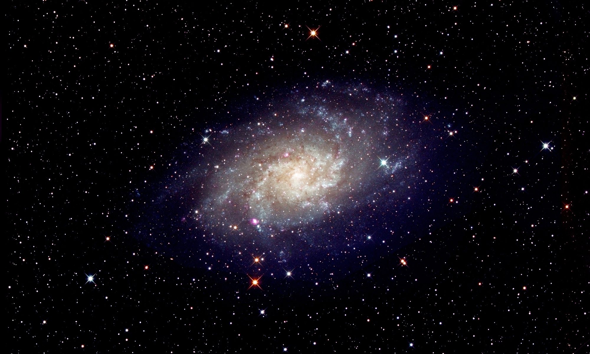
This describes the processing of 30, 20 second exposures taken of the open cluster M41 that lies below Sirius in Canis Major. Though sparse, it is one of the prettiest open clusters in the skies as, amongst the hot blue stars in the cluster, are a number of red giant stars which appear orange in colour. They were taken during some rapid first tests of the (excellent) TS-Optics 90mm f/6.6 triplet APO refractor. The images were captured with an Altair Astro 294C CMOS colour camera.
Calibration Frames – or lack of
No dark, flats or bias frames were taken for this brief imaging test – as none were needed. Dark frames are very useful to eliminate the effects of dark current, amp glow and hot pixels. However, these few frames of M41 were taken from an urban location at a very low elevation, thus the sky noise would totally dominate the noise in the image so the effects of dark current and amp glow would not be apparent. However the effects of hot pixels could still be visible in the stretched final image but stacking software will often remove them. Flat frames allow one to remove the effects of vignetting towards the corners of the frame, but using a Micro 4/3 sensor this would not be apparent. [If there is significant light pollution the image, this (as will be shown) enables a perfect light frame to be produced from the stacked image which can be then be incorporated if the data is aligned and stacked a second time.] If dark frames are taken – as they should be – at the same sensor temperature, exposure and ISO as the light frames then the bias current is included so there is then no need to take any bias frames. [This does not seem to be widely known but, I promise you, is true.]
An introduction to the workspace for those new to Affinity Photo
This section for newcomers to the program and describes those features of Affinity Photo that are used in the tutorial.
The tools palate is a vertical bar on the left hand side of the image space. The required tool symbol is simply clicked upon to activate. Those used in this tutorial are the ‘crop tool’ and the ‘paint brush’ tool that lies below the colour disk.
Across the top of the workspace lie some drop down menus:
In the ‘File’ submenu, one can open and export (rather than save) a file and initiate the aligning and stacking procedure that is available in the 2021 upgrade to the software.
In the ‘Edit’ drop down menu one can ‘undo’ or ‘redo’ adjustments that have been made to the image and also activate the ‘Inpaint’ function.
In the ‘Document’ drop down menu one can convert the format to, say, reduce it’s size or change the bit-depth of an image.
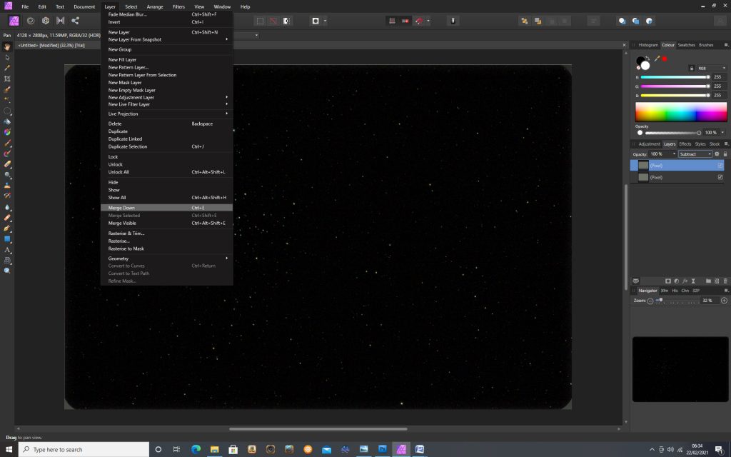
In the ‘Layer’ drop down menu one can ‘Duplicate’ a layer or ‘Merge Down’ two or more layers.
In the ‘Filters’ drop down menu one can go into the ‘Blur’ drop down menus to apply the ‘Median’ blur used when removing the light pollution in the image.
At the top right one can select the colour of the paint brush. Below are a set of adjustment tools. Clicking on, say, the levels tool three options may be brought up; ‘Default’, ‘Darken’ and ‘Lighten’. The default modes are used in this tutorial and, when clicked upon, bring up the tool window. To immediately apply its effect after adjustment, as will be done in this tutorial, one clicks upon the ‘merge’ tab.
The use of layers
When a tool, such as ‘Levels’ is used to alter an image, AP produces an ‘Adjustment Layer’ that sits above the preceding layer and these will build up as more tools are used unless they are ‘merged’ after each tool is applied. Advanced users will keep multiple layers active – which has the advantage that any single adjustment layer can be altered later if desired without affecting any of the other adjustments made. This is quite hard to describe in a tutorial and so I will use the approach where each adjustment layer is merged immediately after its application so only one layer remains active. If necessary, within the ‘Edit’ drop down menu one can backtrack as many steps as one wishes to get back to an intermediate step that one is happy with. At certain points within the editing process I will ‘export’ the current version of the image so that, should I need to leave the program or should it crash, I will be able to continue on from that point. I have found that, occasionally, AP has crashed when, as a novice, I have made some mistakes in using it. On a couple of these occasions, this required a hard reset of the computer. The program also crashed when it somehow ‘disapproved’ of two out of 45 tiff files that I had been attempting to stack. [I had to find them by trial and error.]
Stacking the Image
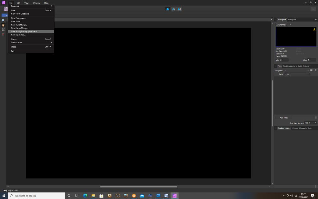
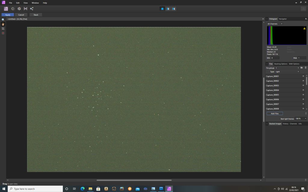
In the ‘Edit’ drop down menu, ‘New Astrophotography Stack..’ is clicked upon and, over to the right of the screen the ‘Files’ input window is brought up with the ‘Light’ subframe type selected. Clicking on ‘Add Files’ one can select the subframes to be aligned and stacked.
Once selected, one clicks on ‘Stack’ at upper left of the screen to initiate the process – which takes quite some time.
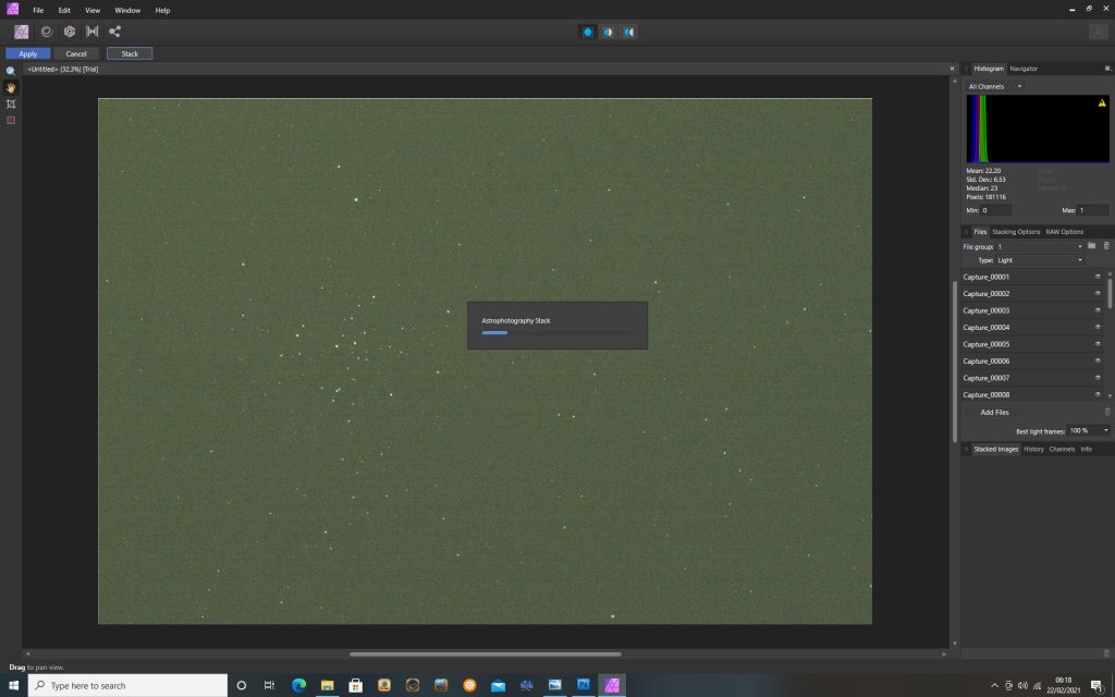
Finally, when completed, on clicks on ‘Apply’ at the upper left of the screen to give the stacked image as a 32 bit file. [The image appears green as the astro colour camera is more sensitive to the green part of the spectrum.]
In case one needs to return to this point, it can be worthwhile to ‘Export’ this file: clicking on ‘Export’ in the File drop down menu brings up a window allowing one to select the format and bit depth of the exported file. (Usually Tiff 16 bit)
Removing the sky glow (light pollution)
Though, in this case, there is no need to process the data in 32-bit depth, this will be left unchanged. The image is duplicated within the layers drop down menu and the upper layer changed to 16 bit within the ‘Document’ pull down layer – convert format.

The ‘Median’ filter (Filters> Blur> Median) is applied with a radius of 90 pixels and the stars, magically, disappear. [Incidentally, if there is a reasonable amount of sky glow (light pollution) in the image, this makes a very good ‘Flat’ frame.]

In the Layers blend mode drop down menu, ‘Subtract’ is selected with an opacity of 100% and then clicking on ‘Merge Down’ in the Layers drop down menu produces an image with a totally black sky background. [Many astophotographers do not like a totally black sky background, so at the end of the imaging process, this can be addressed.]
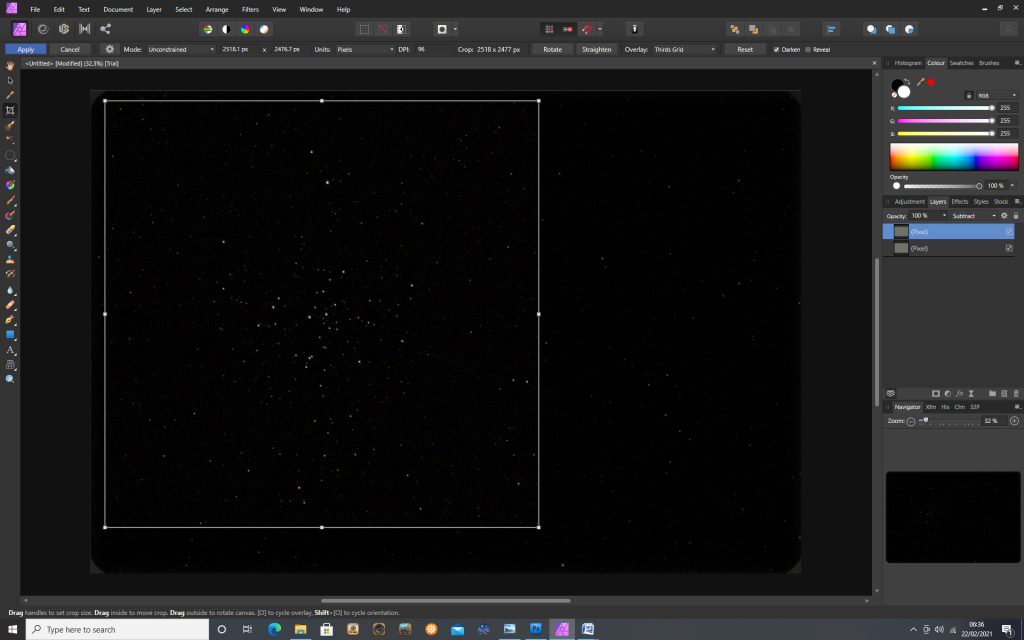
Cropping the Image
The crop tool was selected from the Tools panel at left and the image cropped down to just cover the cluster.
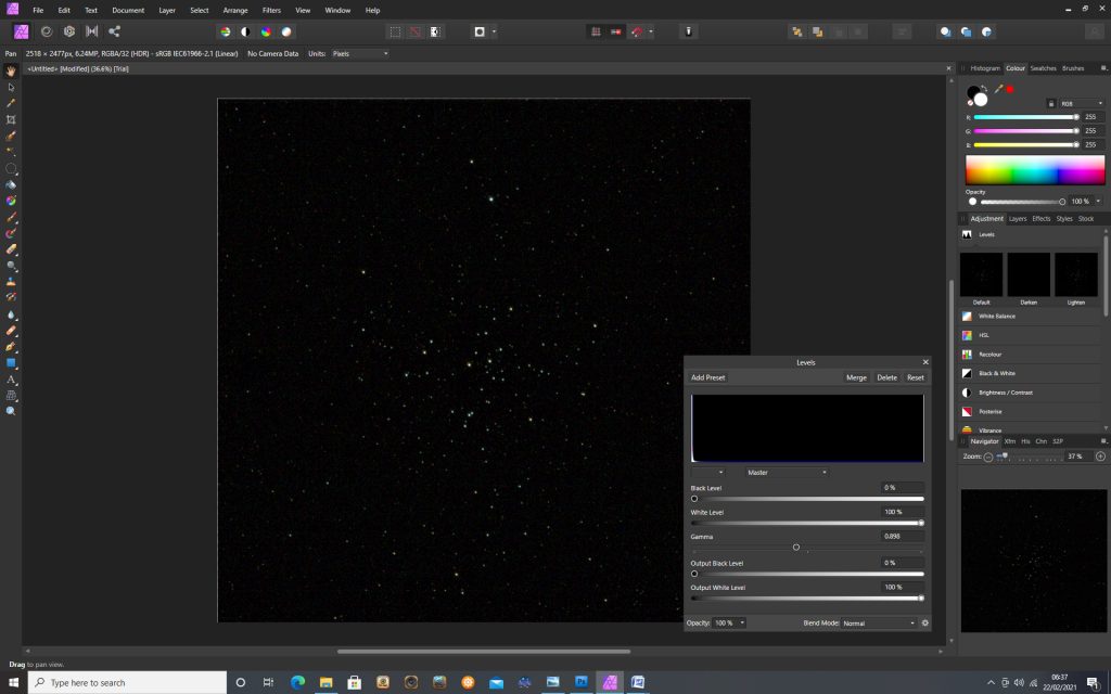
Stretching of the image to bring out the fainter stars
There are several ways of stretching the image one can either use the curves function or, as in this case, the levels/gamma method which works well with this data set.
The image is opened and, in the ‘Adjustments’ panel on left, ‘Levels’ is clicked upon which brings up three small panels. The ‘Default’ levels adjustment tool is opened. Within its window, the gamma slider is moved to give a value of, say, 0.8. One will see that the fainter parts of the image increase in brightness more that the brighter parts – thus producing some image stretching. Two applications allowed the sky background level to become obvious.
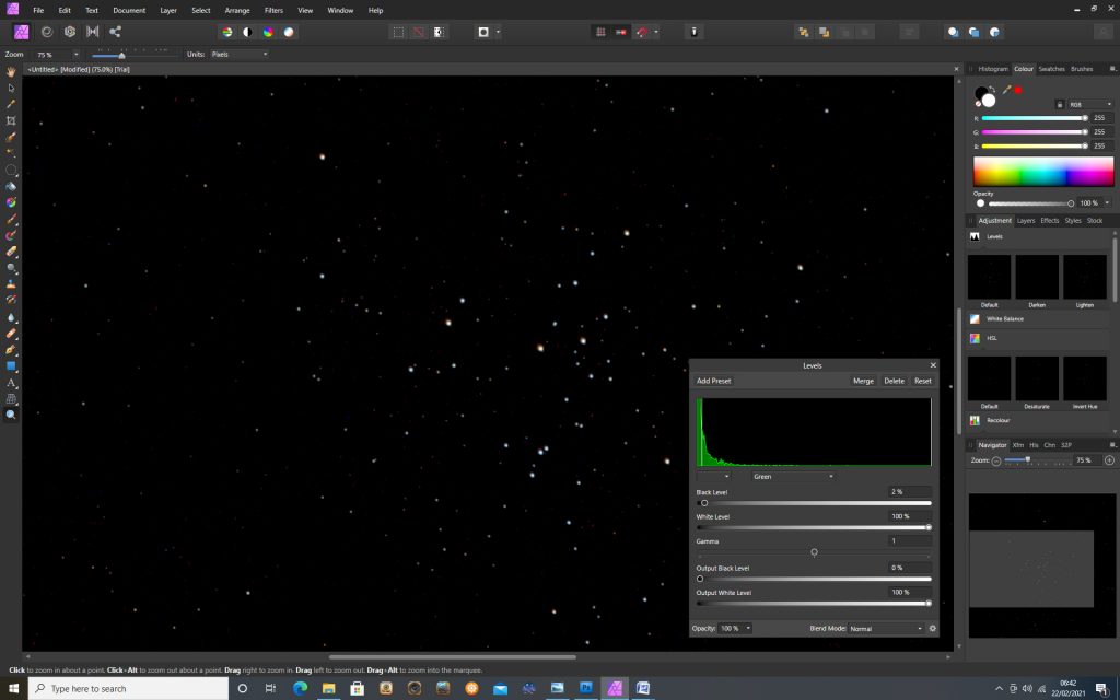
The same ‘levels’ procedure can then be applied again to bring out the fainter stars.
This additional stretching may bring up the background level and use of the ‘black point’ slider in the levels command can reduce this if necessary.
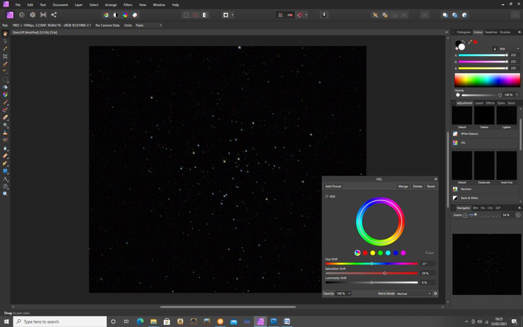
Increasing the colour saturation
The ‘HSL’ adjustment tool is opened up and the saturation slider is moved over to the right to increase the saturation.
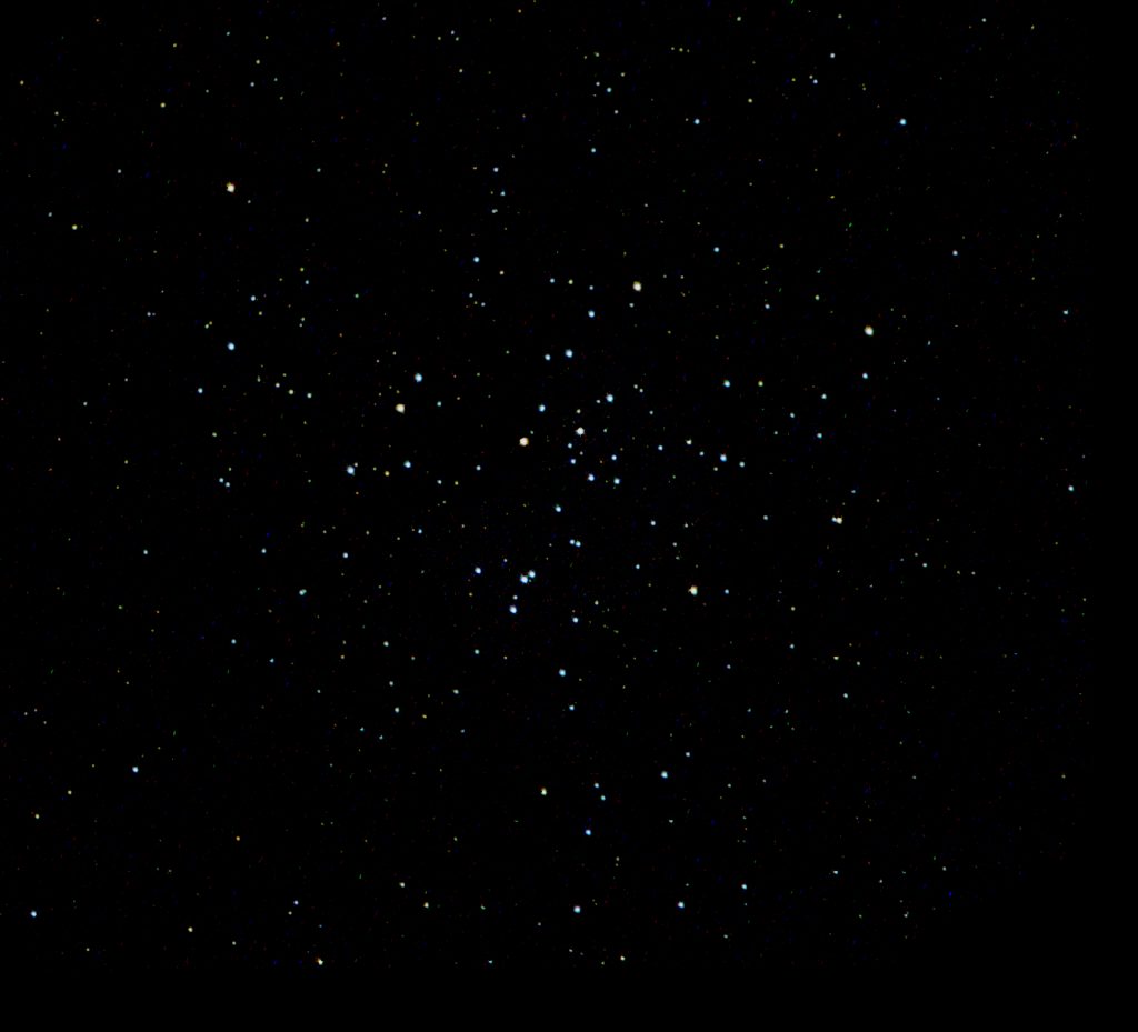
The result:
Adding some background brightness
I desired, one can uniformly increase the sky background to that the sky is not totally black. The image is duplicated and the upper layer is painted a dark grey.
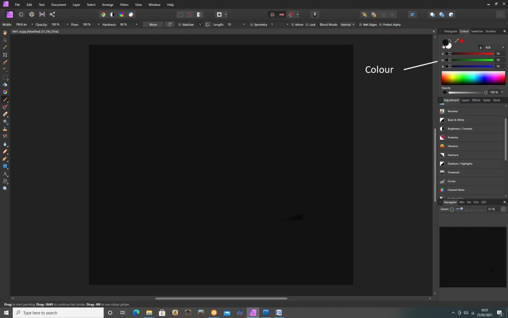
If the layers blending mode is set to ‘Add’, the opacity of the upper layer can be adjusted to a low amount to brighten the sky background and give the final result.
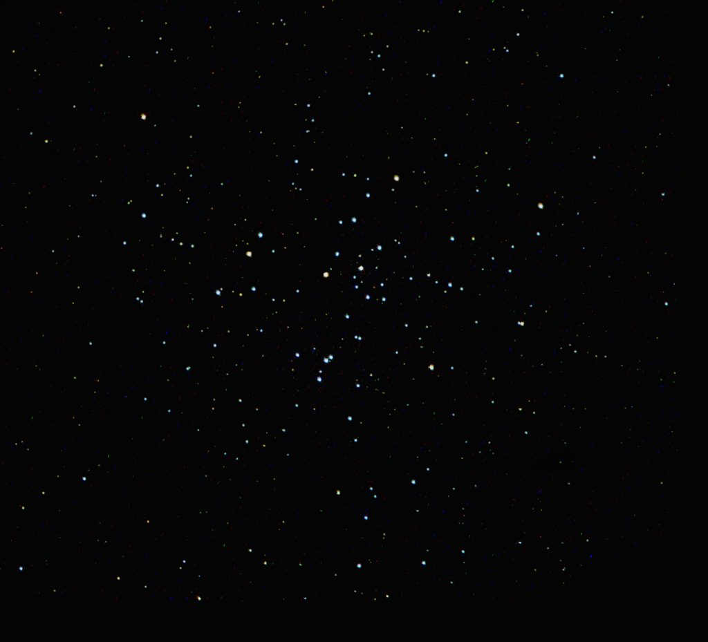
This is not an excellent image as it was taken from an urban location and, as it is at a very low elevations, sky glow will have masked the fainter stars in the cluster. But I hope that it will guide you through the steps required to do better from a dark sky location. It is a very nice open cluster!
[Note: As M41 is at a very low elevation, atmospheric dispersion will misalign the red, green and blue channels of the stellar images – particularly the red. The image can be imported into Registax 6 (free) and pixel adjustments can be made to the Red and Blue channels to align them. In this case the red channel was adjusted by 2 pixels.]