[This is just one of many articles in the author’s Astronomy Digest.]
This article aims to show how, from start to finish, I produced an image of these clusters. It covers many aspects of wide-field imaging and I do hope it would be worth reading.
Camera and lens – Fujinon X-A10 and Sony 35 mm f1/8
Fuginon produce several mirrorless APS-C camera ranges of which the lowest cost (none are cheap) is the X-A range which now include the X-A7 incorporating a 24 megapixel sensor using a standard Bayer filter array. They have no viewfinder but do have a tilting screen so useful when astroimaging and allow for interchangeable lenses. [Fuji produce a range of superb prime lenses such as the XF 23mm f/2 giving an effective 35mm field of view.] My X-A10, 16 megapixel camera, came with the good quality 16-50mm focal length zoom lens. I do not have any additional prime lenses but do have a K&C Concept adapter so that I can mount any of my 7 Sony A-mount lenses in manual mode such as the 35mm f/1.8 lens (50 mm effective focal length) which I used for this exercise as it would nicely encompass the area of Taurus that I wished to image.
One problem with autofocussing lenses is that they do not have an infinity hard stop. When used for astrophotography they will, of course, be used in manual mode but it is surprisingly easy to knock them out of focus. An ideal solution is to focus on infinity in daylight and then ‘tape up’ the focus ring. At night, one can find accurate focus by observing the rear screen of the camera; in focus fainter stars will become visible and this can actually be a better test than minimising the size of bright stars (which one obviously does as well).
Mounting the camera
When using small mirrorless cameras, I mount them using a ball and socket head on a Baader Nanotracker (around £260 and described in the article ‘Three Tracking Mounts …’.) which is about the smallest tracking mount available. It is powered from a separate controller/battery pack using 3 AA batteries – so making it a very convenient tracking mount for taking to dark sky sites. This was mounted on a lightweight Velbon tripod and aligned by eye on the Pole star. I have made a laser attachment for more precise alignment on the North Celestial Pole but do not, in fact, want the mount to be too well aligned. This means that the image will move across the sensor during the imaging period and this helps to remove what Tony Hallas calls ‘Color Mottling’ (he is American) – a variation in colour sensitivity over regions of 10-30 pixels which, if the tracking is perfect, can give rise to variations in the background colour. Of course, the tracking must be sufficiently accurate so that the stars do not trail in the short exposure frames that will be taken. If not removed, this will mean that hot pixels will leave a trail across the image but, as we will see, this is not a problem.
Setting up the camera to take the individual frames
I tend to use relatively short exposures of around 20 to 30 seconds for each frame. Under light polluted skies (as in this example) there is no point in taking longer exposures. In the digest there is an extensive article ‘What ISO to use for astrophotography.’ which should be worth reading. With Sony made sensors (as also used in Nikon, Fuji and Panasonic cameras) probably 400 or 800 ISO will be best but for Canon cameras 1600 ISO may well be better.
Long Exposure Noise Reduction
When taking long exposures cameras will, by default, employ what is called ‘Long Exposure Noise reduction’. Following the taking of each light frame, the camera takes a further similar length exposure (a dark frame) with the shutter closed. It then differences these with the result that hot pixels in the frame will be removed. This is fine when taking a single low light exposure, but not when a large number of frames are to be stacked and aligned to give the result of a long exposure totalling many minutes. Firstly, and most importantly, this will halve the time capturing photons from the sky! Secondly, but not so well known, the process will actually add some noise into each light frame.
[This is why, when capturing dark frames for use when calibrating the light frames, it is suggested that at least 20 are used. This is to average out their noise contribution. The problem with trying to use a set of dark frames captured later is that, in an un-cooled camera, the sensor temperature, and hence the dark current contribution, will increase as a set of light frames is taken.]
The point is that the hot pixels can be removed in the aligning and stacking process, so unless imaging on a very warm summer night, this process should be disabled.
Raw and/or Jpeg capture
The simple rule is to take both! The digest includes an article ‘Could Jpegs be better than raw? …’. Surprisingly, for reasons that are outlined in the article, this can sometimes be the case and is relevant to this imaging exercise.
Exposure time and sequencing
The digest include an article ‘What exposure to use when astroimaging?’ which suggests that, under light polluted skies, individual exposures of ~ 25 seconds will be suitable. The Fuji camera includes a easy to use intervalometer so this was used to take a continuous sequence of exposure. The interval should be set for a few seconds longer than the exposure to allow time for the image to be written to the memory card. The exposure time and ISO were such that, in a single exposure, I could make out both Aldebaran (that lies in front of the Hyades Cluster) and the Pleiades cluster and was thus able to frame the image nicely.
Processing the captured frames
Aligning and Stacking the raw frames.
For this exercise, I used Sequator to align and stack both the raw and Jpeg frames − a total of 52. [The digest includes an article ‘Sequator: a stacking program to rival Deep Sky Stacker’.] Scanning through the Jpegs, I found that a plane had passed overhead and was captured on one frame of the sequence − which was deleted from the stack. (Removing one frame in 52 will have no discernible effect but, with fewer frames, planes or bright satellites can, for example, be removed in Deep Sky Stacker using the Sigma-Kappa combining mode.)
[I found that Deep Sky Stacker was unable to stack the raw files – presumably there were not enough bright stars – but could stack the Jpeg files. This indicates that in producing the Jpeg file from the raw file in camera, some stretching of the image takes place so making the stars brighter. ]
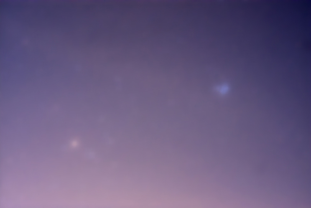
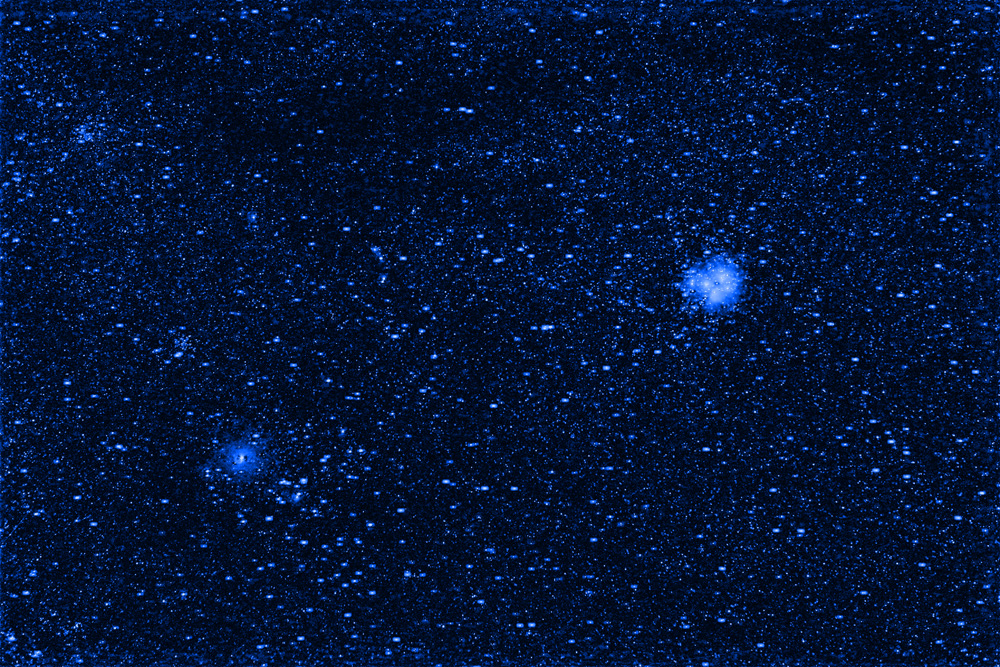
The aligned and stacked result (as a 16-bit Tiff file) was very bright due to the light pollution. Now that our town uses LED street lights, the R, G and B contribution are roughly similar, so as a first step, using the Levels adjustment tool, the left hand slider (which controls the black point) was moved up to the left hand end of the histogram. Having done this the variations in colour across the image due to the light pollution became obvious – the light pollution being more prominent to the lower left which was towards the town centre, 1 mile away.
Removing the Light Pollution
One can buy a program called ‘Gradient XTerminator’ to do this and there is an article in the digest showing how to do this in both Adobe Photoshop and GIMP. For this image I used Photoshop.]
The first thing is to duplicate the image forming two layers. The ‘Noise and Dust’ filter is applied to the top layer with a radius of 50 pixels. The filter thinks the stars are dust and removes them.
The Pleaides, Aldebaran and some other brighter regions are still apparent so, hoping that the light pollution did not vary too quickly across the field, these were cloned out from neighbouring areas. The layer was then smoothed with a Gaussian Blur of 50 pixels radius to give an image of the light pollution.

The two layers were then flattened using the difference blending mode and a little stretching applied.
Hot pixel trails and their removal in Sequator
In the stack made with none of the additional features selected, one can see (in the 100% crop below) the trails produced by red and blue hot pixels. These trails showed how far the image had moved across the sensor. However, by first selecting the ‘Reduce Dynamic Noises’ mode, and then aligning and stacking the frames, these had been eliminated (below).
[The hot pixel trails were 132 pixels long so that the star images had moved ~2.6 pixels across the sensor during each 25 second exposure – not enough to sensibly trail the star images.]
Repairing the red stars
Looking at these ~100% crops it was seen that the brighter stars were surrounded by a red ring. As red light has a longer wavelength, the star images will be larger in the red channel than the blue or green which could have been the case, but I need to investigate this further. This is why that it is important to prevent infrared light falling on the sensor as this would give rise to severely bloated stars. There are several ways to correct this problem. One method is as follows.
Having loaded the image, the channels box is enabled. Clicking on the top right hand corner (very small) menu block, one can select ‘separate channels’. This produces three monochrome images for the Red, Green and Blue Channels. One then needs to note down the image size so that a new blank image can be opened of this size as a 16-bit RGB Tiff image. By opening its channels one sees three blank channels and, if each monochrome image was copied and pasted in turn into the appropriate channel, the original image would be reproduced. But, here is the trick; if the ‘Minimum’ filter (in Filters/Others) with a radius of one pixel is applied to the red monochrome image, the stellar images become smaller. If this, reduced star size, grey scale image is pasted into the red channel of the new image, the result will be that the red bloating will have been greatly reduced. (Clever – and used by many astrophotographers.)
A second method would be to use the Select > ‘Color Range’ tool and sample the deep red ring of the bloated stars and reduce its saturation. One can expand the selection so that the whole of the stars are included and then apply some Gaussian Blur to give the whole star some colour. This makes the stars bigger, so the ‘Minimum’ filter could be used to reduce their size.
Using the Jpeg result
The overall image was quite pleasing but very little of the blue nebulosity in the Pleaides Cluster was visible (as seen in the top left section of the image below). I have found this before and written it up in the digest article ‘Could Jpeg be better than raw…’. So I identically processed the Jpeg data and found that the star bloating was considerably worse. However, the Pleaides nebulosity was far more obvious and was of course captured in the blue channel. So I split the channels to give the three monochrome RGB images and removed the Green and Red images. First I converted the Blue monochrome image to RGB colour rather than monochrome. This image was duplicated and the upper layer was painted blue. The two layers were the flattened using the ‘Color’ (American) blending mode and the faint stars and nebula became blue.
The Pleiades region was cropped out as seen in the top right of the image below.
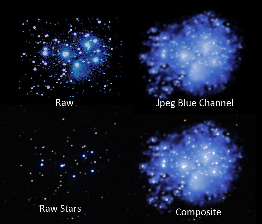
The levels command was used to remove the blue nebulosity from the Pleiades region of the raw result to give the result shown in the lower left of the image. The Blue Jpeg Pleiades crop was then copied and pasted onto the whole image and, with the ‘Screen’ blending mode selected, aligned over the Pleiades (the stars in both could be seen as the position of the Jpeg layer was adjusted) and the two layers flattened.
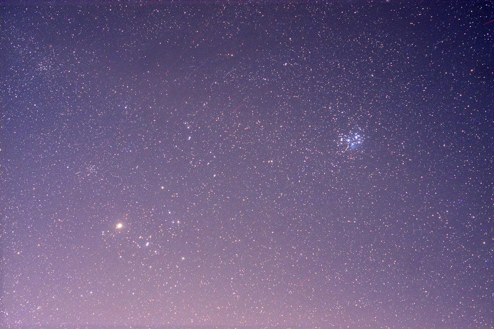
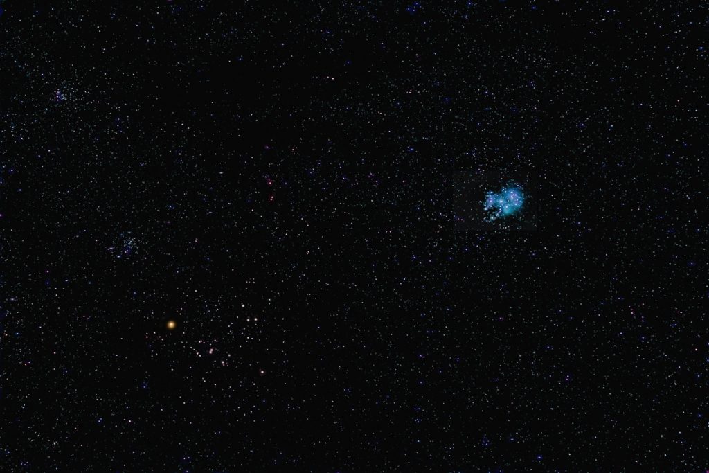
The result was that the blue nebulosity derived from the Jpeg stack was added to the raw derived image, seen below, giving what I think is quite a nice image of the Taurus region.
A higher resolution of this image can be found at:
http://www.jb.man.ac.uk/astronomy/nightsky/Hyades&Pleiades.jpg
First converting the raw files to .Tiff files
In an article ‘Astronomy Digest article ‘Deep Sky Sacker: could it be worth first converting the raw files to Tiffs?’ I suggested that the result of using the Tiff files produced from the raw files might give a better result. I have tried this in this case and found that the Pleiades Nebulosity was a little more obvious than in the straight raw derived image but not as good as that had became visible in the Jpeg result.
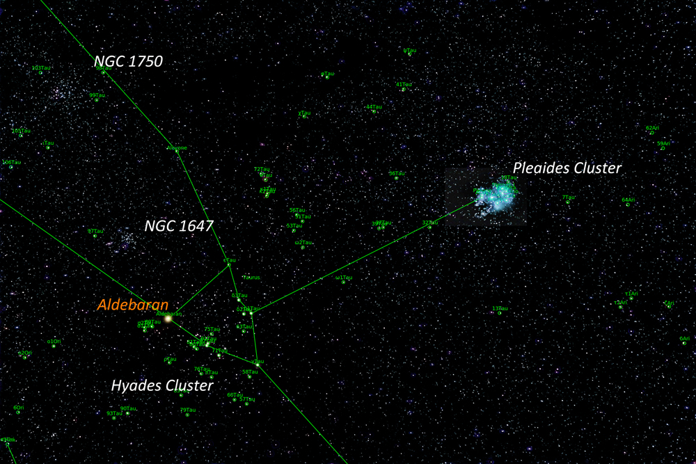
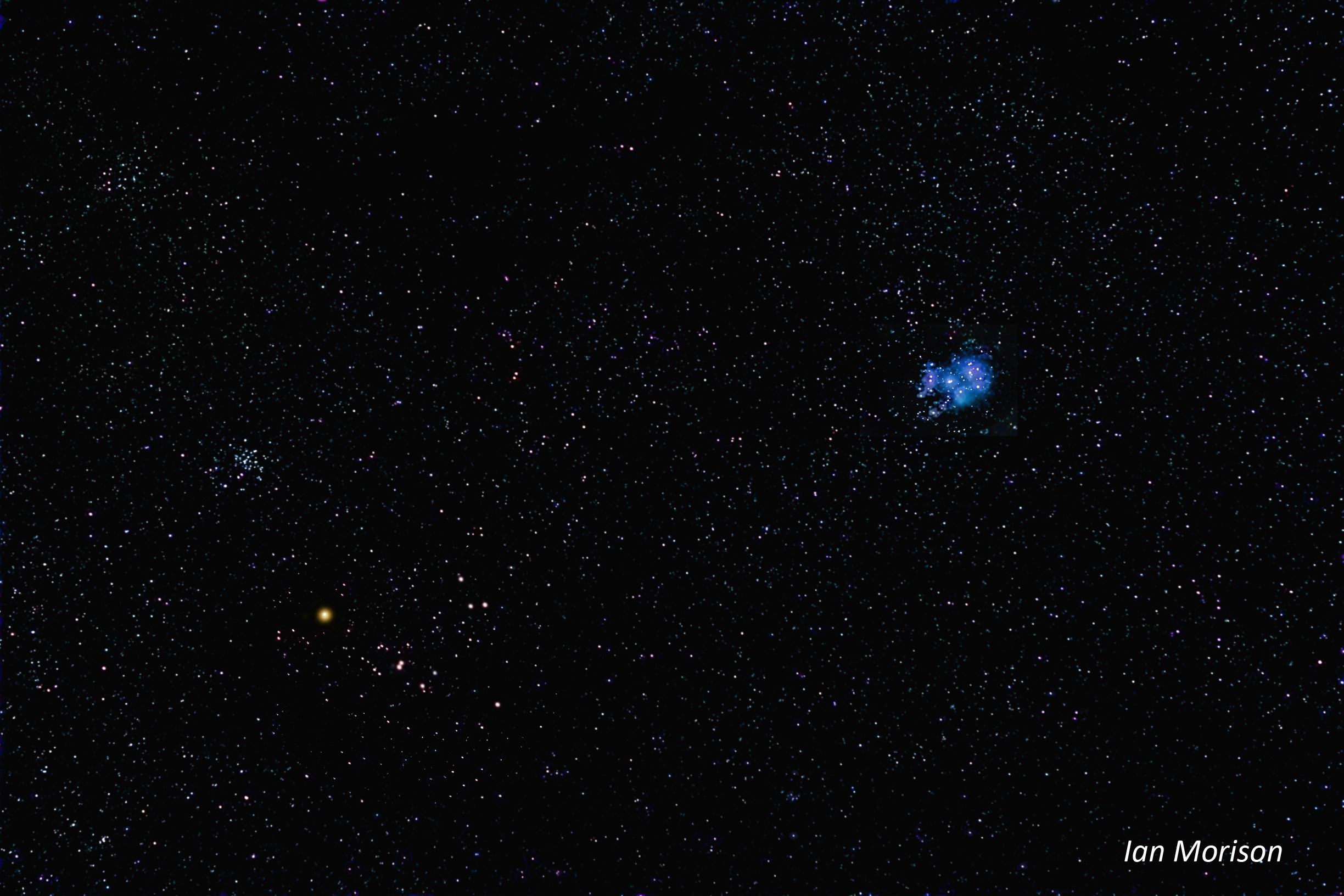
The final image shows the result of ‘platesolving’ the image using the ‘Astrometry.net’ program. The star alignment across the overall field of view is near perfect showing the 35mm Sony lens showed effectively no distortion.