[This is just one of many articles in the author’s Astronomy Digest.]
An example of planetary imaging: highlighting the use of raw video files and the correction of atmospheric dispersion which now affects images of both Jupiter and, particularly, Saturn.
This is, perhaps, the most difficult and, sadly, often a somewhat disappointing astroimaging task. The disappointing aspect is that, from the UK, it is virtually impossible to obtain the crystal clear images such as those taken by Damian Peach using a 14-inch telescope from Barbados where the atmosphere can be exceedingly calm.
The basic idea used for imaging planets is called ‘lucky imaging’. A planetary webcam is used to take many hundreds of very short exposure images, called frames. It is hoped that a reasonable number of these will be taken when the atmosphere along the line of sight is less turbulent than on average and so will be sharper. Processing software then analyses each frame and allows the sharper frames to be aligned and stacked to produce a high quality image. Perhaps naively, I first thought that this process would completely eliminate the effects of the atmosphere. This is not so and really good images will only result when the ‘seeing’ is exceptional. Sadly, this is rarely the case in the UK − which is why Damian Peach goes to Barbados!
The difficult aspect is that of taking the video sequences which will be processed to produce the planetary image. In order to be able to rapidly take a sequence of frames, the number of pixels − and hence the size of the imaging chip in the planetary webcam − must be small to allow the data from the chip to be downloaded fast enough into the control computer. The problem is then to place the planetary image onto the sensor which may only be 4 x 3 mm in size and then keep its image on the sensor whilst the video sequence is being taken. If, as was the case with many webcams, the frame rate was 30 frames per second and a sequence of 2,000 frames were taken, then the sequence would take just over a minute. Unless the mount is accurately aligned on the North Celestial Pole and is tracking well this is a real problem. A very sturdy mount is required!
The latest webcams have both larger sensors, can operate at higher frame rates and may even use a USB3 data link to the computer. The computer, often a laptop, must then be able to ‘digest’ the data stream and save it to disk sufficiently rapidly. When I obtained a (relatively) large sensor webcam I found that though the laptop could buffer the data in RAM, it took twice as long to download this onto its internal hard drive or to an external USB3 hard drive. This effectively halved the total imaging time available. The problem was solved by upgrading the internal hard drive to a solid state disk drive (SSD) and by also acquiring an external USB3 SSD drive.
Using a ‘Flip Mirror’
Even with a well aligned and sturdy mount it is not that easy to place the planetary image onto the webcam sensor. The solution to preventing much anguish is to purchase a ‘flip mirror’ such as those made by Vixen. This is mounted into the 2-inch focuser barrel. With the mirror angled at 45 degrees, the light path enters a 1.25-inch eyepiece. When the mirror is removed from the light path, the image is passed through a Barlow lens (reason for use below) to fall on the webcam sensor. Using first a wide field eyepiece – say 25mm focal length, the planet is acquired and centred in the field. This can then be replaced with a short focal length eyepiece which, ideally, might have illuminated cross-hairs and the planet accurately centred. This eyepiece can usually be made par-focal with the webcam sensor so, having flipped the mirror, a reasonably sharp image appears on the screen of the laptop running the acquisition software. The image can then be accurately focussed and one can begin to take video sequences.
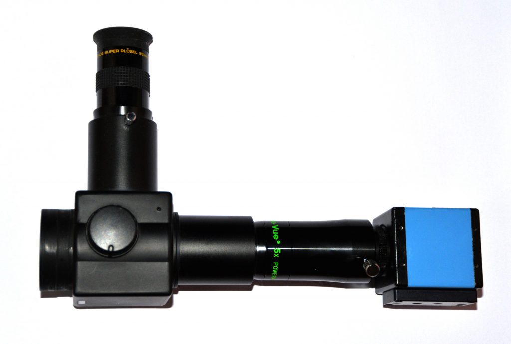
Vixen Flip Mirror, Barlow Lens and planetary imaging webcam.
Why incorporate a Barlow Lens?
Planets, even Jupiter, have small angular sizes and if a webcam is used without a Barlow lens, the image on the sensor (dependant on the focal length of the telescope) may be so small that the image is not well sampled by the array of pixels in the sensor. Let’s take an example: suppose one was imaging Jupiter which, near opposition, has an angular size of ~44 arc seconds. One might (optimistically) hope to achieve a resolution of one arc second under excellent seeing conditions and so, to sample the image sufficiently, the Nyquist theorem states that the image scale of each pixel should be no more than half an arc second and preferably a third of an arc second. There should thus be at least ~88 pixels across the planet’s disk.
A Barlow lens is thus incorporated to increase the effective size of the planetary image. However increasing its image size will reduce its brightness so that longer exposures will be necessary to capture each frame. The longer the exposure, the less likely that ‘sharp’ images will be captured and so a compromise has to be reached.
When the ‘maths’ are done it turns out that under typical conditions a telescope/Barlow combination should have an effective focal ratio of ~20. This takes into account the fact that larger aperture telescopes (which collect more light) can have longer effective focal lengths. Thus a x2 Barlow would be used with a typical f/10 Schmidt-Cassegrain. For the 127mm, f/7, refractor employed to take the Jovian image described in this essay, I used a x2.5 TeleVue Powermate to give an effective focal ratio of f17.5. This was just about sufficient, as there were 80 pixels across the Jovian disk, nearly reaching the Nyquist criteria. [As it turned out, the seeing limited the overall resolution of the final image to ~3 arc seconds so the Nyquist criteria was easily met.]
If the atmosphere is particularly calm − so longer exposures can be employed − then a greater effective focal ratio can be used. So then perhaps an effective focal ratio of f/30 to f/35 might well be used.
Colour or Monchrome webcam?
If a monochrome webcam is used, a set of three video sequences captured through red, green and blue filters is required, so a filter wheel and set of filters is needed. In principle, this provides the maximum possible resolution that can be obtained with a given sensor but there is a problem with Jupiter and Saturn in that, due to their fast rotation rate, the sequences must be completed within a few minutes otherwise blurring will take place. Damian Peach suggests that one takes a sequence R-G-B-G-R so that the blue .avi is used twice and two images are obtained.
The far simpler alternative is to use a colour webcam where each pixel is covered with either a red, green or blue filter called a Bayer matrix. For each 2×2 grid of pixels, 2 are sensitive to green, and one each to red and blue. Thus the nominal resolution, given the same size image on the senor, is halved. To overcome this problem by doubling the image size would require longer exposures so probably giving lower quality resulting images in any case. However it is much simpler to use a colour camera and I would advise any but an accomplished imager to use one.
In fact, the effective resolution may not, in fact, be halved if the planetary image is allowed to very slowly move across the webcam sensor. Unless the mount is perfectly aligned this will be the case anyway and I always very slightly misalign my mount so that the image moves by perhaps 20-30 pixels during the taking of a video sequence. There are two advantages: the effects of any dust spots on the sensor will be mitigated and the resolution can approach that when using a monochrome webcam. The reasoning behind this is complex, but some justification can be given by the fact that some Olympus cameras have a ‘high resolution’ mode where the sensor is shifted by very small amounts whilst 8 exposures are taken over a ~1 second period (a tripod must be used). These are then combined and, even though employing just a 16 megapixel sensor, it can output an effective 40 megapixel image! One can see the results at the : Olympus High Resolution Imaging Mode website.: Olympus High Resolution Imaging Mode. Allowing the planetary image to move very slowly across the sensor whilst perhaps 1,000 or more frames are taken may have much the same effect.
So let’s continue assuming a colour webcam is to be used.
RGB or raw data capture
There are a number of ‘codecs’ that can be used when capturing the video frames to make a .avi file. One can capture uncompressed colour images where, for each pixel, 8 bits are used for each colour. With a typical 640 x 480 pixel array this would require ~300,000 bytes (~0.3 megabytes) per frame hence a 1,000 frame sequence would require ~300 megabytes. Either the camera itself or the capture software will have to ‘deBayer’ the raw data captured by the sensor as, of course, each pixel only produces one monochrome 8-bit data word. For speed, they will often use a rather crude deBayering algorithm called ‘nearest neighbour’ which for every pixel colour takes the colour of the nearest pixel having that colour filter above it. If the data is compressed then far smaller files will be produced as much of the captured image will be black! But, to be honest, this is not the best way to capture planetary images.
Save raw data
It is far, far better to record uncompressed raw data. The codec is called Y800 when an 8 bit data word is captured for each pixel. No processing is required in real time, so faster frame rates may be possible: with the Imaging Source DFK21AU04.AS that I use, the capturing of raw data allows a frame rate of 60 frames per second rather than 30 when an RGB .avi file is taken. Even more importantly, it is possible for each frame’s data to be deBayered later using far more sophisticated algorithms such as ‘HQLinear’ which is found within the ‘deBayer.exe’ program that is bundled within the free ‘Firecapture’ program. [Firecapture is now used by many imagers when using webcams to capture planetary images.] Very pleasingly, deBayer.exe’ can also reduce the size of the output file by centring the planetary image within a smaller pixel area. This obviously takes time in post capture processing, but as a smaller pixel area is produced, the following analysis software may run more quickly. This latter technique also helps when the planetary image is rotated at the end of the imaging process so I would recommend its use.
Imaging Jupiter at low elevation and in bad seeing conditions
As a processing example, I imaged Jupiter in April 2017 with a 127mm apochromat refractor, Vixen Flip Mirror and a x2.5 TeleVue Powermate to increase the effective focal ratio to f/17.5. An Imaging Source DFK 21AU04.AS colour planetary webcam was used to capture the video sequences. The seeing was poor and Jupiter’s elevation was not high so dispersion in the atmosphere affected the final image. Not surprisingly, the result is not as good as the example included in ‘The Art of Astrophotography’ which was captured when seeing was better and Jupiter was at a high elevation but it does give an idea of what ought to be able to be achieved under typical conditions in the next few years from the UK.
Capturing the video sequences
The data provided by the Imaging Source webcam was captured with IC Capture 2.4 (Imaging Source’s proprietary capture software) using the Y800 raw codec. Video sequences of 1-2,000 frames were captured. The figure below shows three typical frames of one sequence along with the aligned and stacked image produced by the video processing program.
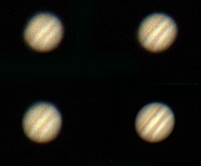
Three frames (having been deBayered) and the stacked image of ~1,200 frames.
DeBayering the raw video file
The .avi files produced were deBayered using the HQLinear algorithm within DeBayer.exe and, at the same time, a smaller file is made by outputting a smaller pixel array centred on the planetary disk. One has to ‘tell’ the program the layout of the filters overlaying the individual pixels (there are 4 possibilities) and a choice is given. If the default pattern is wrong, the image will have a false colour. For my Imaging Source colour webcam, the pattern is ‘GBRG’ and one thus selects the ‘GB’ pattern. The following figure show the first frame as deBayered by deBayer.exe with, above, the full captured frame and, below, the area of the frame when the program outputs a smaller pixel area. This .avi file is smaller that the original raw file and so the original file can then be deleted if one wishes to save the data long term.
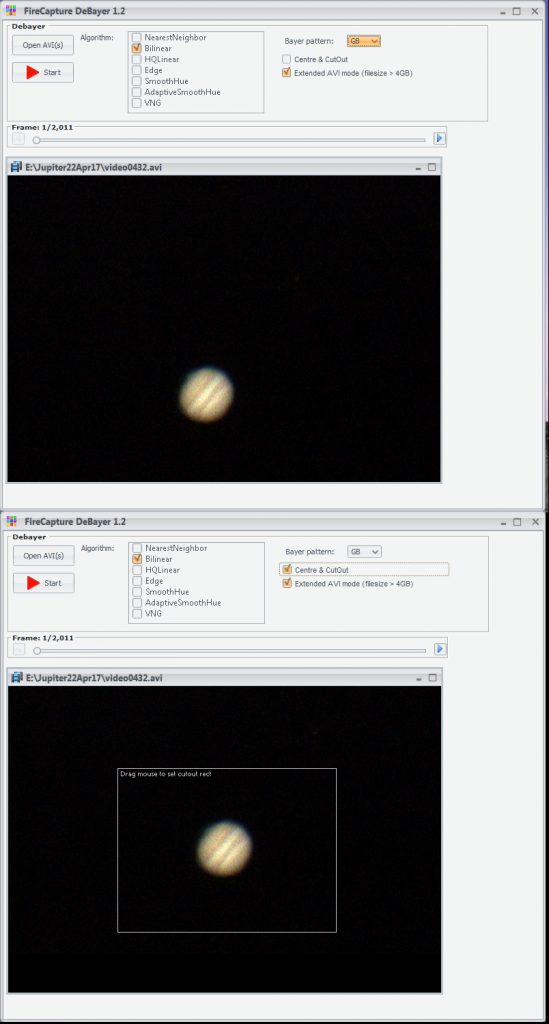 DeBayer.exe screens showing the first frame when, above, the full image area is to be processed and, below, a smaller pixel area centred on the Jovian disk.
Processing the colour video file
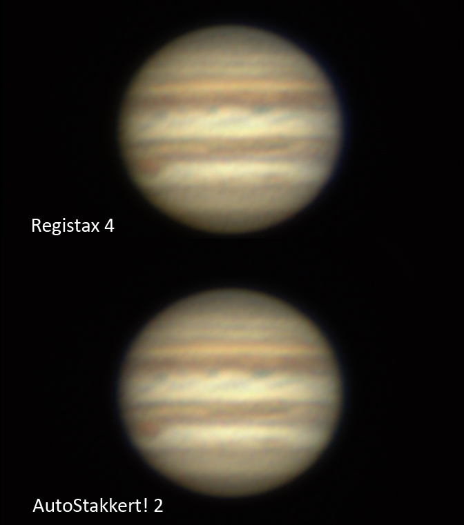
One now has a colour .avi file which has to be processed. There are two main programs designed to achieve the production of a good planetary image; Registax and Autostakkert! 2. The top flight imagers are now tending to use Autostakkert! 2 but I (not being top flight) have, in the past, felt happier using an early version of Registax. The current version is Registax 6 but, using the earlier version, Registax 4, I can ‘watch’ the sequence of processes being carried out and feel that I have more control over the processing. This can still be downloaded for free from the Registax website. So I will first outline how I use Registax 4 to process a planetary .avi file. It has to be said that processing the video file is far quicker in Autostakkert! 2 and this is also described below. The final figure compares the result of processing a single video file with the two programs – I fail to see any difference between them – but Autostakkert! 2 automatically carried out the atmospheric dispersion correction and its sharpened version (two images can be provided, one sharpened) was excellent. So perhaps I will try to join the top flight imagers and use Autostakkert! 2 in future!
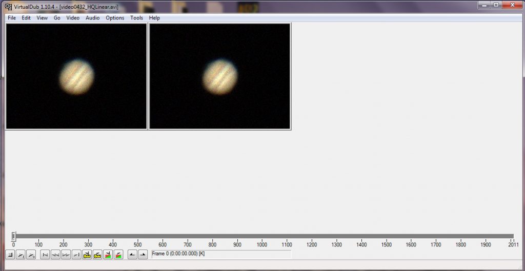
The Virtual Dub program
Sometimes it is found that the processing programs cannot open the .avi files output from the capture software. If so, the Virtual Dub program can often produce a .avi file that can be opened. The file is opened and, when the F7 key is pressed, a new .avi file is made (which can be given a suitable name) and placed in the folder where the original file was found.
Using Registax 4 to process planetary images
Registax 4 will accept a Y800 raw file but then uses the ‘nearest neighbour’ method of deBayering which can produce artefacts. [Read my article about this is the digest.] This is why I use DeBayer.exe to carry out the production of the colour .avi file. The Registax program is opened and the .avi file selected at which point the first frame appears on the screen. Moving the green cursor below shows successive frames and one will see how the image is moved and distorted by the atmosphere. It is then best to use the curser to select one of the better frames.
The alignment options tab is clicked upon and one can select the size of a bounding box that will just cover the planetary disk. (In the case of the worked example, this was 128 pixels across.) At this point, a window appears showing a somewhat garish image which is the fourier transform of the planet. The parameter at bottom right is adjusted (usually by increasing the number to ~8) so that there is no colour visible in the corners of the frame. In the case of Jupiter, I like to see some striations across the frame due to the equatorial bands across its disk.
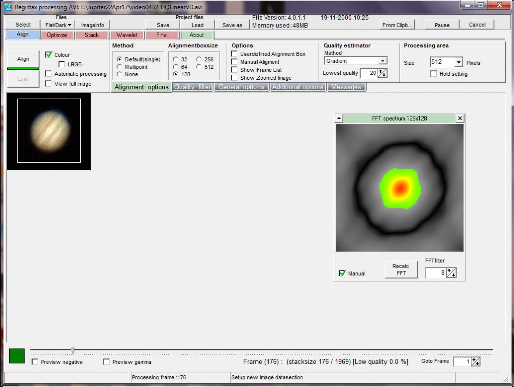 The opening screen of Registax 4: a bounding box has been placed around one of the better frames and its fourier transform shown.
Aligning the frames
This is a two stage process, first an approximate alignment is carried out and then an ‘optimising’ process is carried out. The ‘Align’ tab is clicked upon and one sees the bounding box following the planetary image across the sensor. One gets a good idea at this point as to how good the seeing was − little random movements across the sensor and relatively undistorted images indicate good seeing. [If deBayer.exe has produced a file with a smaller area, one will not see any slow movement across the sensor as the program will have already carried out an approximate alignment.] Registax has then ranked each frame in terms of image quality and has measured their X and Y positional offsets (in pixels) from the initially selected frame. At this point the ‘Limit’ tab is clicked upon. If the full fame is being analysed a green line appears showing a measure of the overall movement across the frame. If deBayer.exe has output an approximately aligned smaller pixel area, nothing is seen at this point.
The next step is to ‘optimise’ the alignments. To achieve this, a ‘reference’ frame is produced from some of the sharpest images: the ‘Create a Reference Frame’ tab is clicked upon and one sees the program stack some of the sharpest frames to give a reference image which is displayed to the left of a single frame. One then clicks first upon the ‘Continue’ tab and then upon the ‘Optimise’ tab and a plot is constructed showing the displacements of each frame from the reference frame. Usually two passes are made but one could limit this to a single pass by clicking on the ‘Single run optimiser’ box.
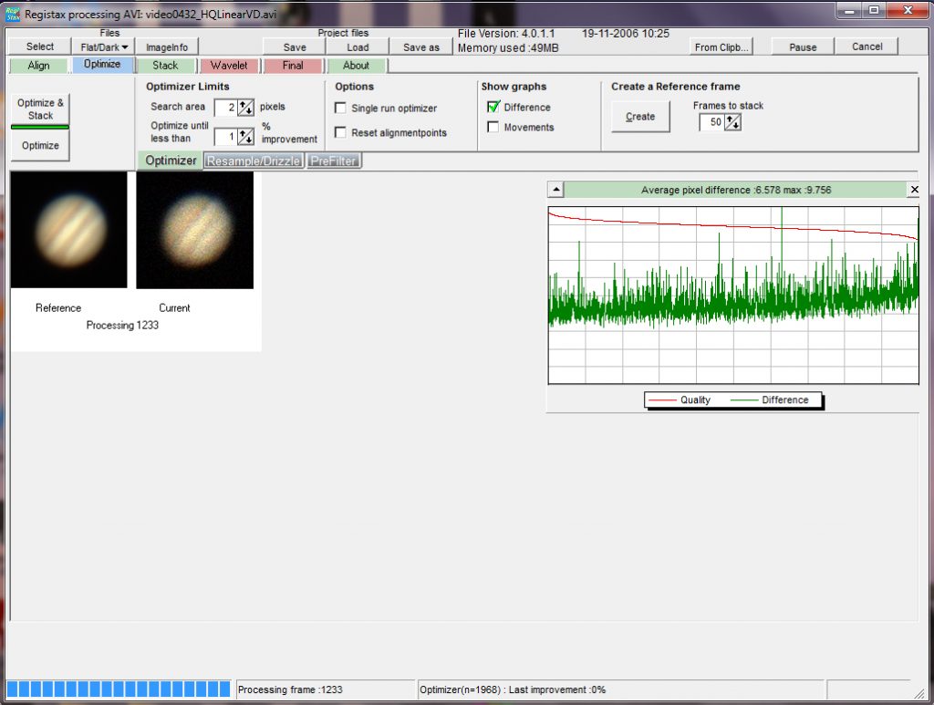 Having carried out the optimisation process.
This complete, the small ‘Stack’ tab in the top row (not the large one at the left) is clicked on and the ‘Show Stackgraph’ box ticked. A window then shows all the frames ordered from left to right in rank order. The grey slider below the graph is then moved to the left to remove the less good frames from the stack and the slider at the top left of the window is moved down to remove those frames whose offset errors were more than most as shown in the figure below. This is where some judgement is required. Selecting just the sharpest few frames to stack will give a sharp but somewhat noisy result. Selecting the majority of frames would give a less sharp but also less noisy result which might well allow more sharpening to be carried out after stacking. This is a case where some trial and error is required. If the quality as percentage of the best only falls slowly across the set (with good seeing), one could stack more frames than if there where a rapid fall off in quality. Stacking those down to the 80% level would be a good starting point. The consensus seems to be to stack more rather than fewer frames.
 Using the Stack graph to limit the number of frames that will be stacked to provide the unsharpened image on left. 1,248 frames have been selected to be stacked.
This procedure selected 1,248 frames of the initial 1,969 frames which were then stacked by clicking on the large ‘Stack’ tab. Having stacked the frames, the screen then shows the stacked image which should show little noise but be rather ‘soft’.
 Having stacked the 1,248 frames.
Sharpening the image using the Wavelets tool
A great feature of Registax is that it contains a superb sharpening tool that is uemployed even by those that have used Autostakkert2! to align and stack the .avi file. So, at this point, the ‘Wavelets’ tab is clicked upon which brings up a window showing a set of 6 sliders at the left of the stacked image. By moving these sliders to the right, the image is sharpened. A good starting point would be with all values set to 5-10 but there is great scope for trial and error to give a good result. When pleased with the result, the ‘Do All’ tab must then be clicked to apply the sharpening to the whole image before it is saved as a 16 bit Tiff file.
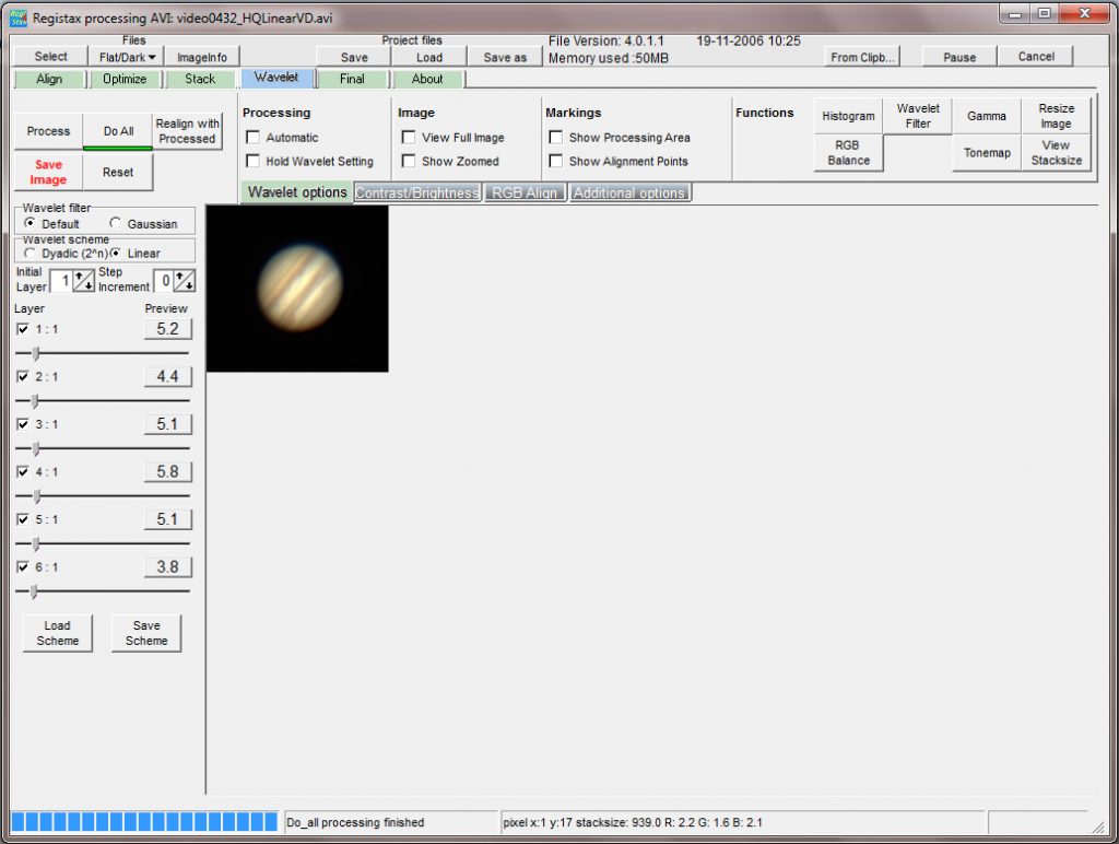 The wavelets tool has been used to sharpen the image.
Compensating for the effects of atmospheric dispersion.
Jupiter and, even more so, Saturn are now well down the ecliptic and so never reach high elevations even when transiting due south. Their images are thus likely to show some red and blue fringing at the top and bottom of the image (if imaged due south) due to dispersion in the atmosphere. In ‘The Art of Astrophotography’ I describe the ZWO Atmospheric Dispersion Corrector which can make the best possible correction but otherwise there is a software tool in Registax 6 that can be used to provide an approximate (but still very useful) correction.
To make it easier to make the dispersion correction, I first increase the size of the image by 400%. This does not, of course, show any more detail, but it makes the dispersion more obvious and a little easier to correct.
The image is then imported into Registax 6. Over to the right are a set of tools, the centre one being ‘RGB align’. This is clicked upon and it is then possible to adjust the positions of the red and blue channels, pixel by pixel, to align them on the green channel. ‘Do All’ is clicked upon and the corrected image is exported as a 16 bit Tiff.
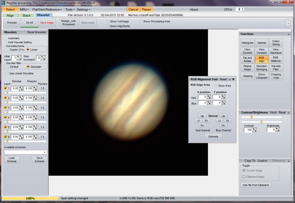 The upscaled image has been imported into Registax 6 and the RGB align tool selected. The effects of atmospheric dispersion are obvious.
 Having aligned the red and blue channels over the green channel.
At this point I will rotate the image so that the equatorial bands are horizontal. [It is important that the rotation is about the centre of the planet otherwise a distorted image results. The planet image must first lie at the centre of the frame (this should be the case if deBayer.exe has centred the image) and perhaps the canvas size increased somewhat. In Photoshop, the frame is selected (Ctrl A) and in the ‘Edit’ menu first ‘Transform’ and then the ‘Rotate’ tool selected. A marker is shown (which should lie at the centre of the planet) and, if the cursor is placed just outside one of the corners, it can be used to rotate the canvas as desired.
One could then, perhaps, tweak the image somewhat. Using, for example, Photoshop one could perhaps apply some local contrast enhancement by using the ‘Unsharp Mask’ filter with a radius of say 100 pixels and a small amount. Perhaps a little further sharpening could be applies using the ‘Smart Sharpen’ filter and an adjustment of the brightness using the ‘Levels’ tool. The Gaussian Blur filter with a small radius (say 1 pixel) might finally smooth the image somewhat.
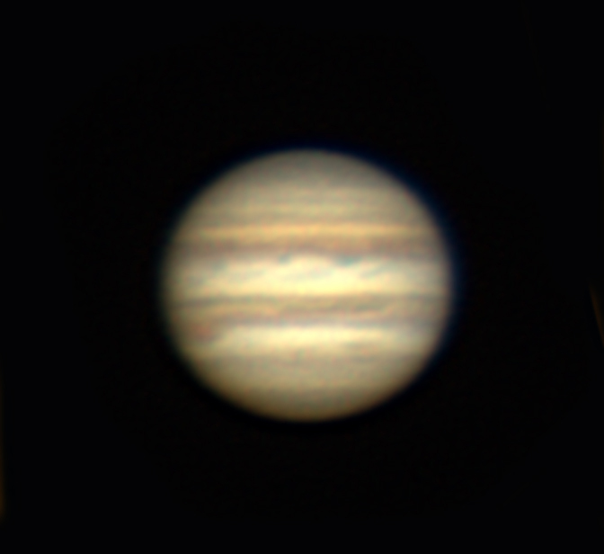
The result of applying some minor adjustments in Photoshop.
As the resulting resolution was not that high, it was possible to slightly improve Jupiter’s image by stacking the results of three successive video sequences taken over four minutes. A total of ~3,000 of the better frames from the three sequences went into the final image.
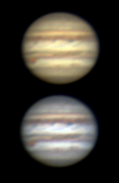
A slightly improved image combining the result from three successive video sequences. The lower image has had ‘Autocolour’ applied to give a white rather than cream overall colour.
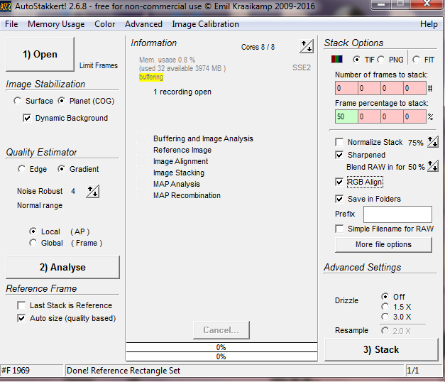
Processing planetary videos in Autostakkert! 2
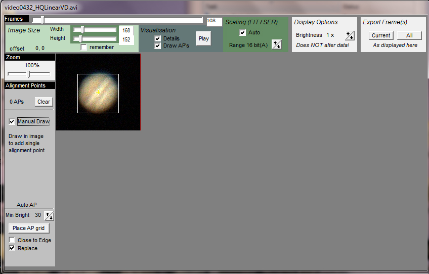
This is a very quick process! When the program is opened two windows appear. The first, shown below, allows one to set some of the imaging parameters such as the percentage of frames that will be stacked (in this case I set it to the best 50%), the fact that I wanted the program to apply a correction for atmospheric dispersion and that I wanted a sharpened image produced as well as the unsharpened image.
The video file was opened and the first frame appeared in a second window, shown below. The cursor at top was moved to the right to select one of the better frames, in this case frame 108 and, having clicked on ‘Manual Draw’ I used the mouse to draw a bounding box around Jupiter so I was setting a single alignment point.
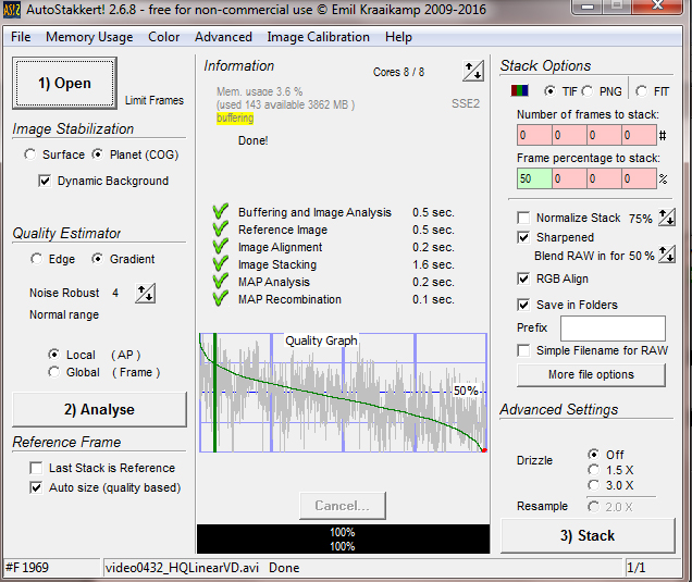
In the first window, the ‘Align’ tab is clicked upon and a plot then appears showing a plot of the frames ranked in order from best to worst.
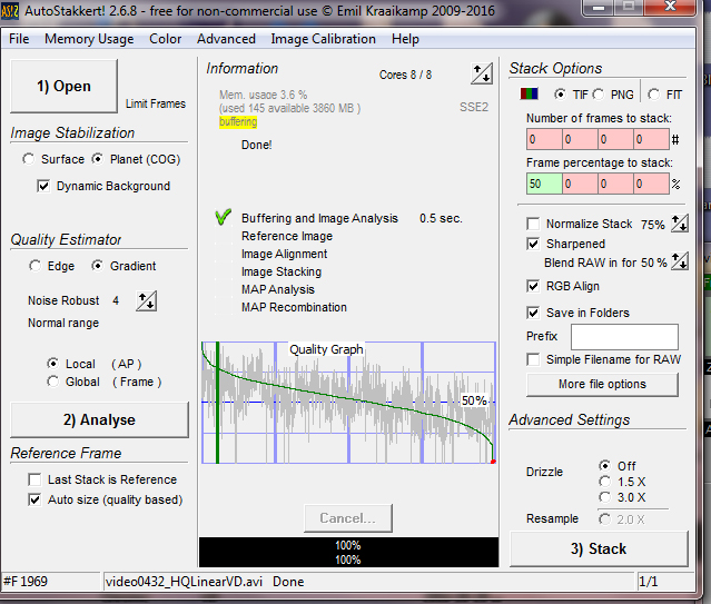
One then simply clicks on the ‘Stack’ tab and it thinks for a short while (using an Intel i7 processor) and gives the times taken to carry out the several processes involved.
As I have requested a sharpened image as well, both images are placed within a new folder made within that which included the video file that was processed. Both are shown below in their original orientation.
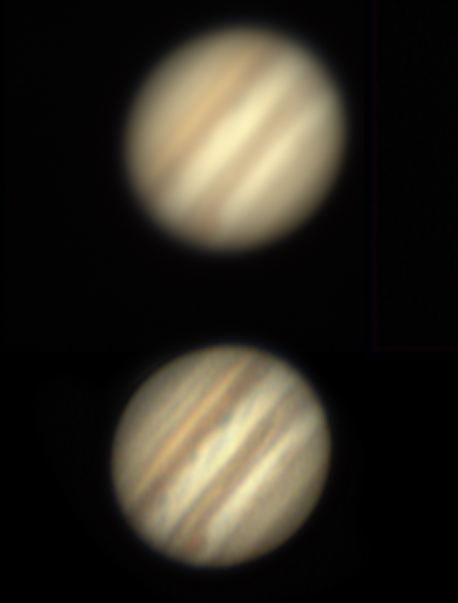
I have rotated the sharpened version and compared it to that produced by Registax 4 (having had some some minor tweaks in Photoshop) in the figure below. I find it hard to find any significant differences so it appears that Autostakkert! 2 did a very good job in a very short time. So I suppose my advice should be first use Autostakkert! 2 but if you are not happy with the result then try Registax 4.
You should be able to achieve an image at least as good as this using 5 or 6-inch telescopes. Using my 127mm refractor to image Mars in excellent seeing conditions along with a x5 Powermate to give an effective focal ratio of f/35, I was able to achieve a resolution of ~1 arc second as shown in the final figure − so it is possible!

Mars imaged at closest approach when just 15 arc seconds across. Below is the WinJUPOS diagram showing what should have been be visible at the time the image was taken. The agreement is excellent and I believe, perhaps surprisingly, it appears that the resolution is slightly better than 1 arc second which is the nominal resolution of the telescope − giving some confirmation that a colour webcam may not loose much in resolution to the use of a mono webcam and filters.