[This is just one of many articles in the author’s Astronomy Digest.]
The article has been amended with a second imaging attempt described at the end.
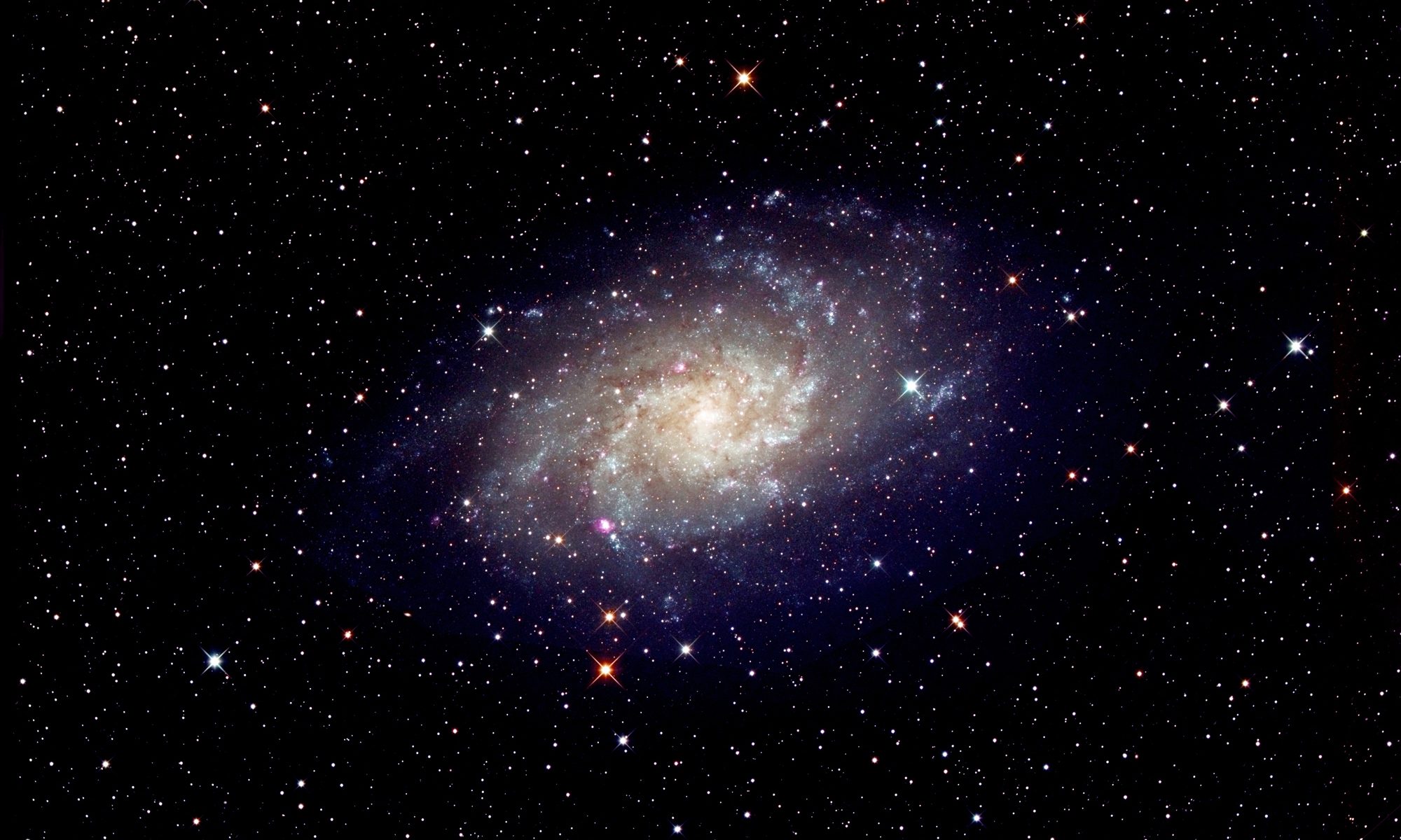
Several times a year, members of my astronomy society spend a weekend or more at a dark site on the north-east coast of Anglesey having unobstructed views to the south and south-west. On Friday 18th May we were blessed with a wonderfully clear sky – albeit not getting dark until 11pm or so! Using Sky Safari I had seen that the Virgo cluster of galaxies would be visible in the south-west after dark and decided to attempt to image part of the Virgo cluster. As it covers a substantial area of the sky I wanted to image with the widest possible field of view that my telescopes and cameras could provide. The obvious choice for a telescope was the TS 65 mm, 4 element, astrograph which is reviewed elsewhere in this digest. This is designed to cover a full frame (36 x 24 mm sensor). My only full frame sensor is within my Nikon D610 camera so this was used. Perhaps as the telescope is designed for imaging, it is the only refractor that I have which will come to focus without having to use a focuser barrel extender. Being an astrograph using a FL-53 element in a triplet objective and a singlet field flattener part way down the optical tube, it should provide pin-point stars across an unvignetted field of view. It does not quite achieve the latter but is pretty close.
The ‘Field of view calculator’ in Astronomy Tools
(https://astronomy.tools/calculators/field_of_view/)
provides an excellent way of checking the field coverage of a telescope/camera combination. This shows the result when using a Nikon D750 (which has the same full frame sensor as my D610) and centred on Virgo A, M87, the brightest galaxy in the cluster.
The field of view calculator screen
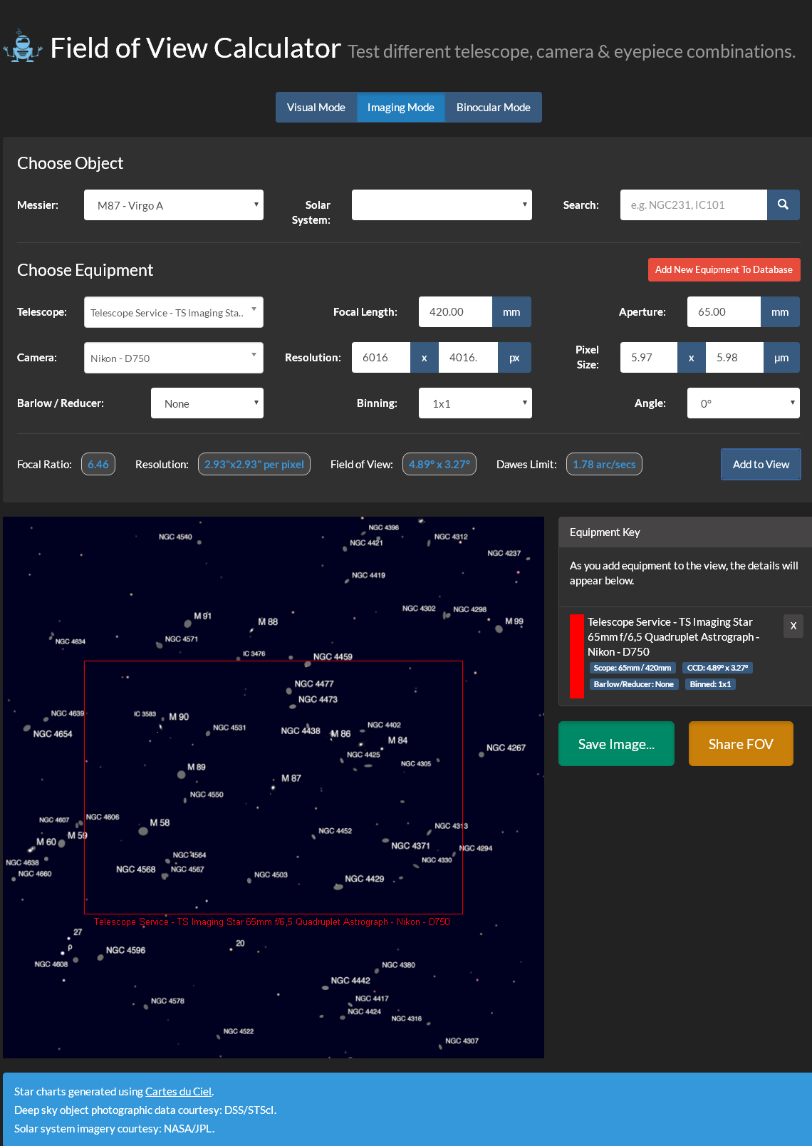
The Field of View Calculator with M87 in the centre
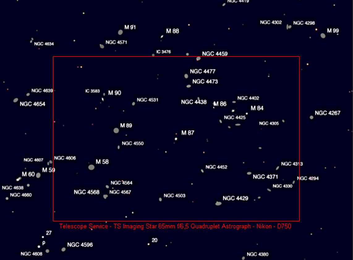
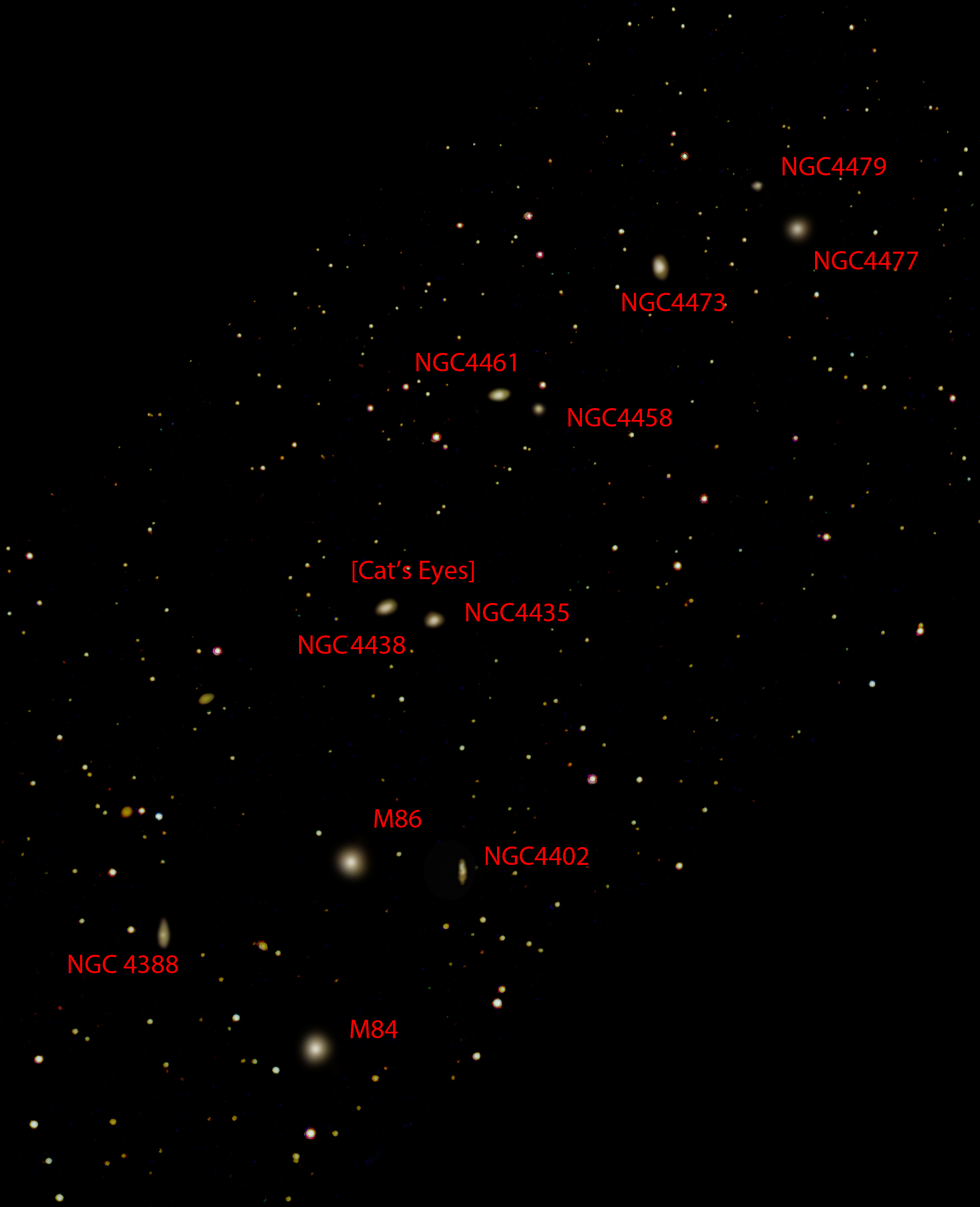
Detail of the region centred on M87
As described elsewhere in the digest, I controlled the camera using the DSLRdashboard App on my Samsung tablet. This acts as an intervalometer and, with a full screen live display, makes focussing easy.
The choice of mount was easy – my iOptron Minitower. It is small and compact, has a built in GPS system to set the location and time, and, once aligned, has excellent ‘GOT0’ ability as will be proven later. This really is a superb ‘Get up and Go’ mount and is described in detail elsewhere in this digest. There is, of course, one down side in that it being an alt/az mount it will suffer from ‘frame rotation’. The program ‘Deep Sky Stacker’ which I use to align and stack the frames will automatically ‘de-rotate’ frames before stacking so that the only consequence is that parts of the image towards the edges will have had somewhat less exposure.
Jupiter was in the south and made an excellent object on which to align the mount. The mount has to be aligned due south with the telescope vertical. I only knew the approximate direction of south but this was no problem. I ‘selected and slewed’ to Jupiter which, as expected, was not in the field of view using a 2-inch wide field eyepiece. However, the elevation should be correct and so slewing the mount in the appropriate direction in azimuth immediately brought Jupiter into view. Having centred Jupiter in a higher power eyepiece, I then ‘synchronised’ the mount to the object. [Parking the mount will then park it facing due south, so an accurate direction south can be found.] Using a 65 mm aperture telescope with a focal length of just 420 mm, the image of Jupiter and its moons was pretty small in the frame but 4 moons could be seen with Io just beside Jupiter’s limb.
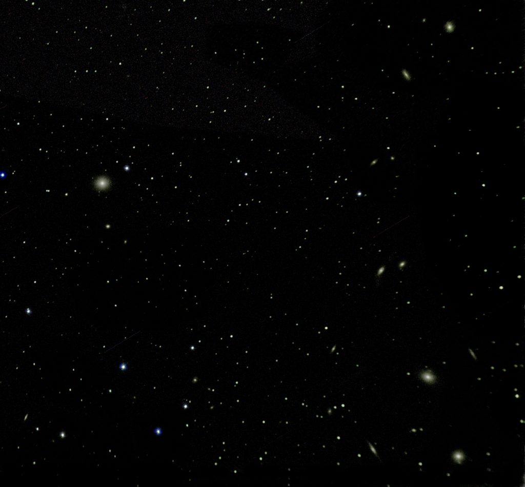
Remembering that Virgo A (a radio source which is the 87th member of Messier’s catalogue) is the brightest galaxy in the Virgo cluster I then slewed to M87. [It was pleasing, that when the final image was aligned and stacked, M87 was near dead centre in the frame.] It was still not dark in imaging terms and so, not surprisingly, test exposures showed a considerable amount of blue in the image. I did not use the ‘in-camera dark subtraction mode’ as this would have reduced the imaging time by half nor did I take any dark frames. Happily, the D610 does have a very low noise Sony sensor. The digest includes a detailed discussion of the use of dark frames when using compact system cameras or DSLRs and it does suggest that, in summer, one should use ‘in camera dark subtraction’. However, I suspect that the added noise to the image was probably dominated by the skylight which, of course, the subtraction of dark frames would not remove. If this were so, the only real effects of using the ‘in-camera dark subtraction’ would have been to add some noise into each frame as well as halving the imaging time. [The fact that subtracting a single dark frame introduces some noise is why one is advised to take 20 or more dark frames which are then averaged by Deep Sky Stacker. The problem with using an uncooled DSLR is that the sensor temperature will increase over the half an hour or so during the taking of the set of frames so one does not know at what temperature one should take a set of dark frames. This is why I recommend using the in-camera method as the dark frame temperature will be very close to the previous light frame – but do read the article!]
I then set DSLRdashboard to take continuous 30 second exposures. Imaging continued until M87 had become obscured by buildings in the south-west. A total of 67 frames had been captured in raw and Jpeg from the time that darkness ‘fell’.
I did point out that the TS refractor does exhibit a little vignetting in the extreme corners which can, of course, be corrected by using a set of flat frames. I had produced a number of flat frames taken earlier when it was quite light. These were converted to monochrome and imported into Deep Sky Stacker along with the light frames.
The 67 frames were then de-rotated, aligned and stacked in Deep Sky Stacker using the average stacking mode. The histogram produced of the result, as seen in the screen shot below, was unlike any that I have seen before. From my light polluted home location, I have a red peak to the right but, for this image, the peak to the right was blue – due, of course, to the residual light in the sky as true ‘Astronomical Darkness’ would only exist for an hour around 1 am BST − well after these frames had been taken. This light is still a form of light pollution and will thus have obscured the fainter outer parts of the Virgo galaxies.
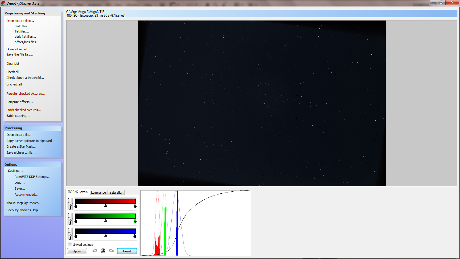
The output from Deep Sky Stacker
When stretched, the pass of a satellite was seen across the image. There are two ways this can be removed. If, instead of the average stacking mode, the ‘Median Kappa Sigma’ mode is selected it will remove any pixels that veer too far from the average. This does, however take some processing time and the alternative which may well be quicker is simply to scan all the JPEG images and find the one with the satellite present. (If it is apparent in the final image, it will be fairly obvious.) I did this and simply deleted it so it would not figure in the averaged stack.
A little stretching was done in ‘levels’ with the central slide moved left to the 1.20 position as shown in the screen shot below. This was made an ‘action’ so could be then achieved with a single (function) key stroke.
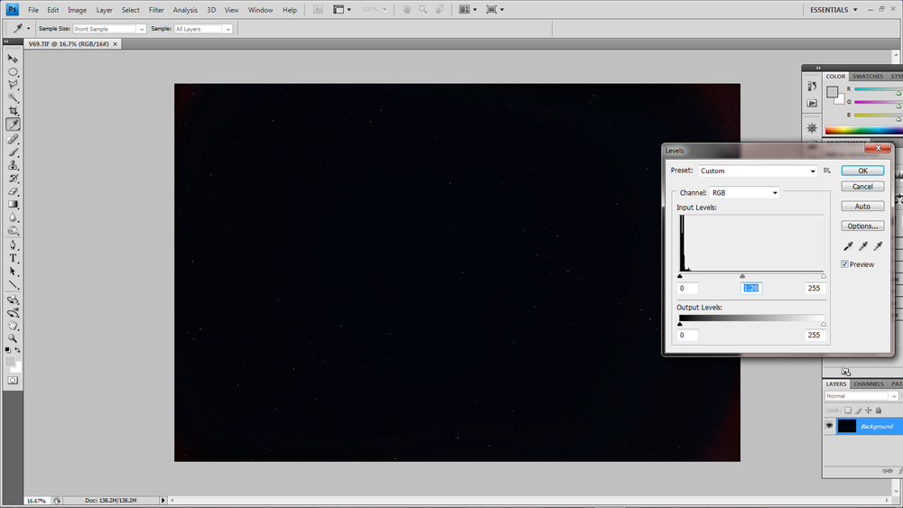
Stretching the output from Deep Sky Stacker
The blue skylight became obvious and to remove it, the image was duplicated and the ‘Dust and Scratches’ filter applied with a radius of 24 pixels. This removed the stars and galaxies leaving just an image of the skylight which was then removed from the initial image by flattening the two images using the ‘Difference’ blending mode. The resulting image could then be stretched a little more.
A technique I have used (as with some others) when imaging nebulae such as the Andromeda Galaxy or the North America Nebula is to separate out the nebula and stars into two frames, enhance the nebula by increasing the ‘local contrast’ of the image and then, using the ‘Screen’ blending mode put back the stars into the nebula image. However as the image is of the nebula, not the stars, using the ‘opacity’ slider one can reduce the star’s brightness somewhat so that the nebula stands out better. In this image, I have made a mask which covered the areas surrounding each of the visible galaxies, inverted it (so that the galaxies were not included in the mask) and then reduced the brightness of the stars. This allowed the galaxies to stand out better from the star field.
Markarian’s chain of galaxies are close by to M87 and its members were visible in the image. Wikipedia states:
‘Markarian’s Chain is a stretch of galaxies that forms part of the Virgo Cluster. When viewed from Earth, the galaxies lie along a smoothly curved line. Charles Messier first discovered two of the galaxies, M84 and M86, in 1781. The other galaxies seen in the chain were first mentioned in John Louis Emil Dreyer’s New General Catalogue, published in 1888. It was ultimately named after the Armenian astrophysicist, Benjamin Markarian, who discovered their common motion in the early 1960s. Member galaxies include M84, M86, NGC4477, NGC4473, NGC4461, NGC4458, NGC4438 and NGC4435.’
This first imaging exercise of the region encourages me to use a longer focal length telescope and cooled CCD camera to image just the region of Markarian’s chain from a dark location in late February or April during astronomical darkness. One should then be able to bring out some of the fainter outer regions of, for example, the galaxy M86 – but this will have to wait until next spring.
A second attempt
The field of view calculator suggests that a good pairing would be to use my 80 mm, 500 mm focal length, refractor allied to my Altair Astro 294c colour camera.
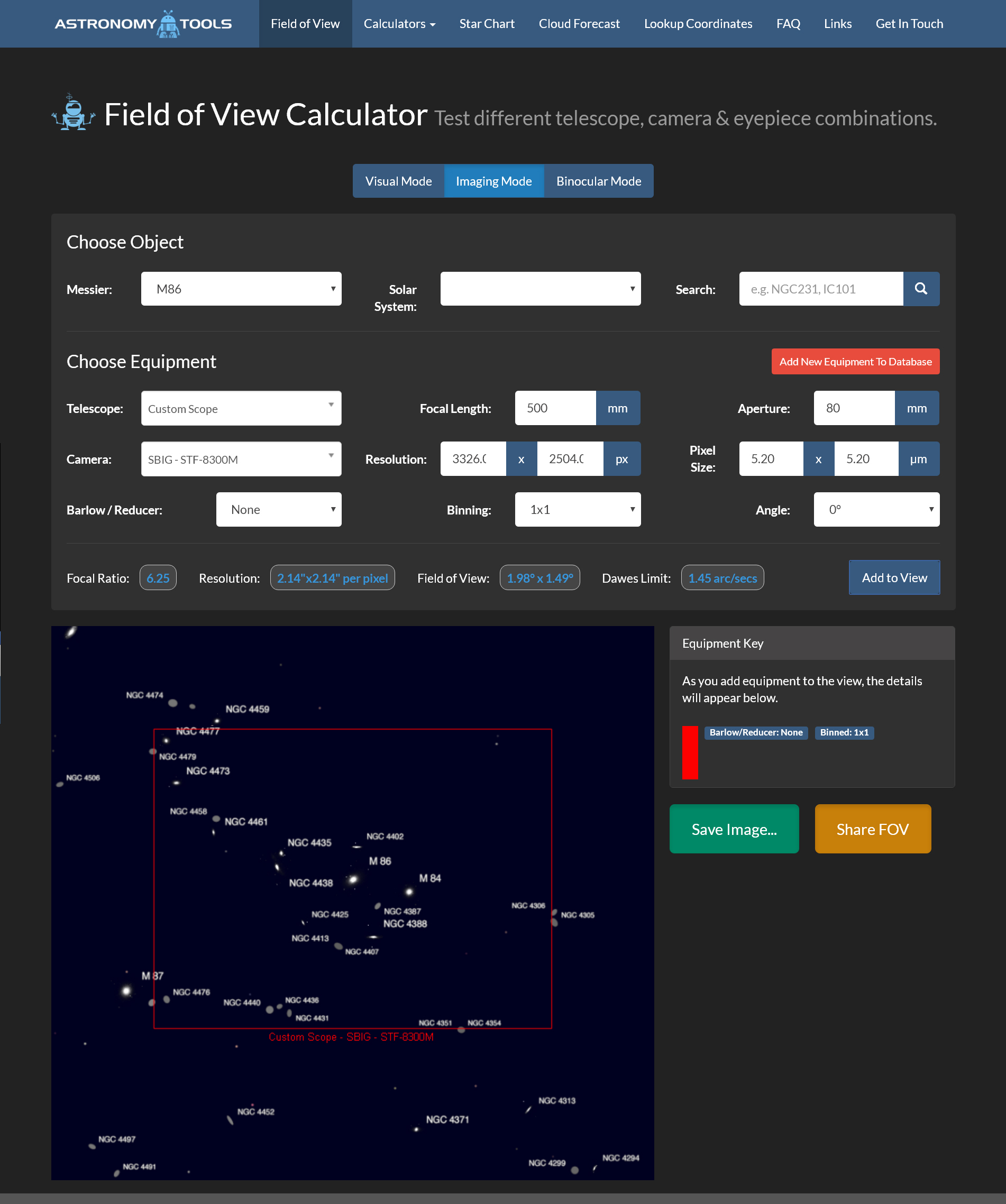
Field of View Calculator with 80 mm refractor and SBIG CCD camera
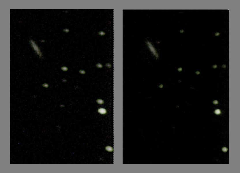
However, in order to do a comparative test of astro cameras, I was asked to use my 80 mm, 400 mm focal length, guide telescope – which is a simple achromat and thus exhibits chromatic aberration. Also a field flattener was not employed so stars towards the edge of the field showed the effects of coma. Happily, this simply elongated the stars away from the field centre and, as shown, is easy to correct. The AA294c is more sensitive to the green so the result has a green cast.
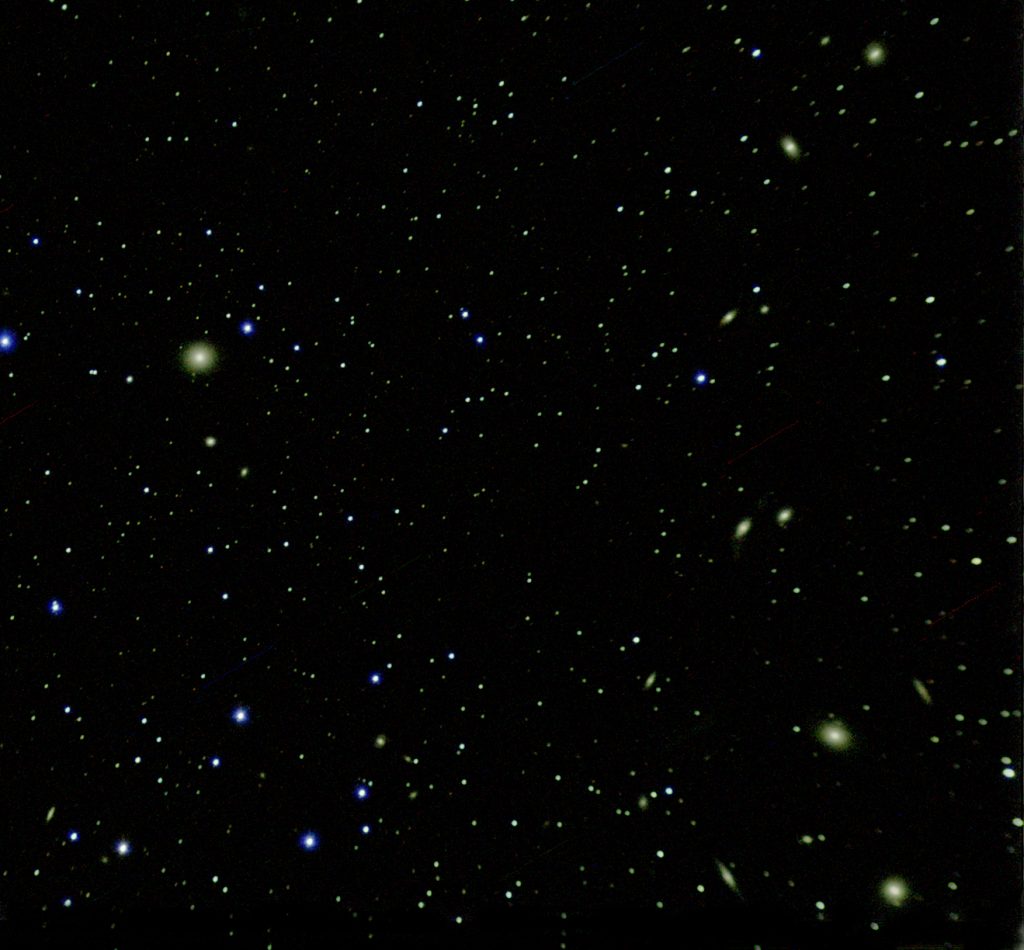
However, the result from stacking 1 hours worth of subframes when the transparency was very poor was able to be turned into a passable image as will be described below.
The result of aligning and stacking in Deep Sky Stacker was stretched in Adobe Photoshop (Affinity Photo could also be used) to give the result below.
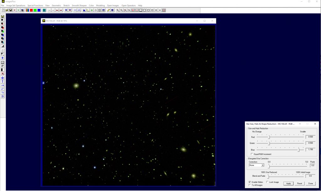
The, now free, software package Images Plus has a good way of dealing with this. In its special tools menu it has a tool to reduce star sizes. One would normally reduce the size of all three colours by the same amount, but one can decouple them and simply reduce the blue channel – which nicely reduces the effect of the chromatic aberration.
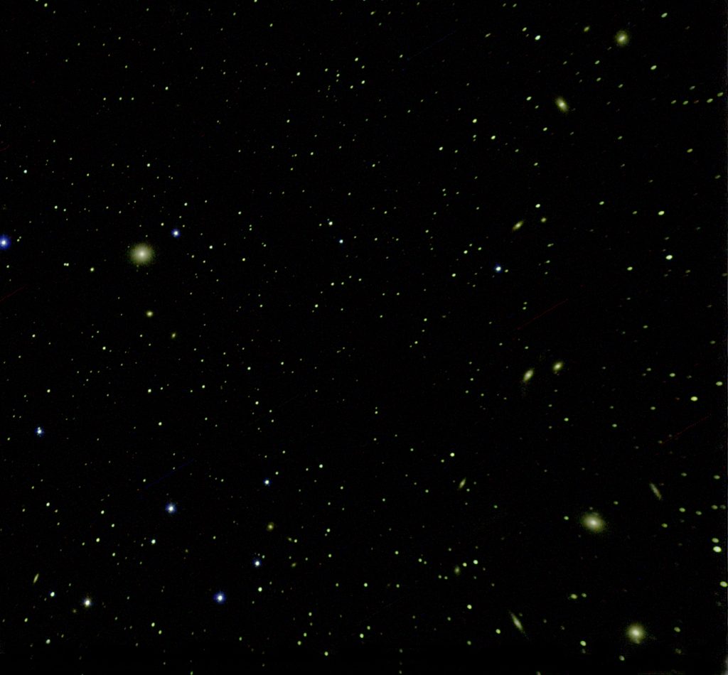
Using the colour balance tool in Adobe Photoshop or Affinity Photo one can reduce the green excess.
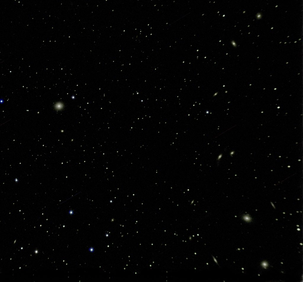
Over to the lower right of the image the coma has elongated the stars (as elsewhere in the image). To correct for this, one can select the problem region, duplicate it, set the layer blending mode to darken and select the ‘Move Tool’. The image must be clicked upon before using the arrow keys to move the upper layer over the lower.
The result is acceptable, but it would have been a far easier to process image having used my semi-apo 80mm refractor and field flattener. It has, however, illustrated a couple of useful processing tools.