[This is just one of many articles in the author’s Astronomy Digest.]
I would not normally consider imaging under partial cloud cover with clouds moving quickly across the field of view but actually this is not quite as stupid as one might first think. The clouds trap much of the light pollution, so imaging through a gap in the clouds can reveal darker that usual skies. I was wanting to try out a newly acquired camera, purchased second hand at low cost, along with an adapter to allow my Nikon prime lenses to be used with it. The camera was a Sony A5000, now quite old but sporting an excellent APSC sized sensor. [Note: In the digest article about Cameras and lenses, I do recommend the newer Sony A6000 for use when a lightweight imaging system is desired.] The Nikon to Sony E-mount adapter cost £35 including postage and, with its use, I was able to mount a Nikon, f/2.8, 55 mm macro lens. This is one of the sharpest prime lenses that Nikon have ever made and, stopped down to f/4 on an APSC rather than full frame sensor, it is near perfect. It has a ‘fixed’ infinity stop so making it easy to set for astroimaging – one advantage of using vintage prime lenses!
The camera was secured on a heavy ball and socket head attached to an Astrotrack which was itself mounted on a Manfrotto tripod using a ‘Junior Geared Head’. This can be used to easily make very small adjustments to the azimuth and elevation of the Astrotrak’s polar axis thus making it very easy to align on the North Celestial Pole – using a laser pointer rather that its polar scope. This could be easier than using an equatorial wedge.
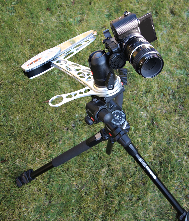
The camera was set to allow the use of manually focused lenses and, in the manual imaging mode, was set to take 30 second exposures at an ISO of 800. The camera was set to save both raw and jpeg files. [It is far easier to scan though a series of jpeg frames to see those that could be used to stack, usually using the raw frames, in a program such as Deep Sky Stacker.] It was linked by wifi to an Android tablet using a simple App, TimeLapse, acting as an intervalometer to initiate its exposures.
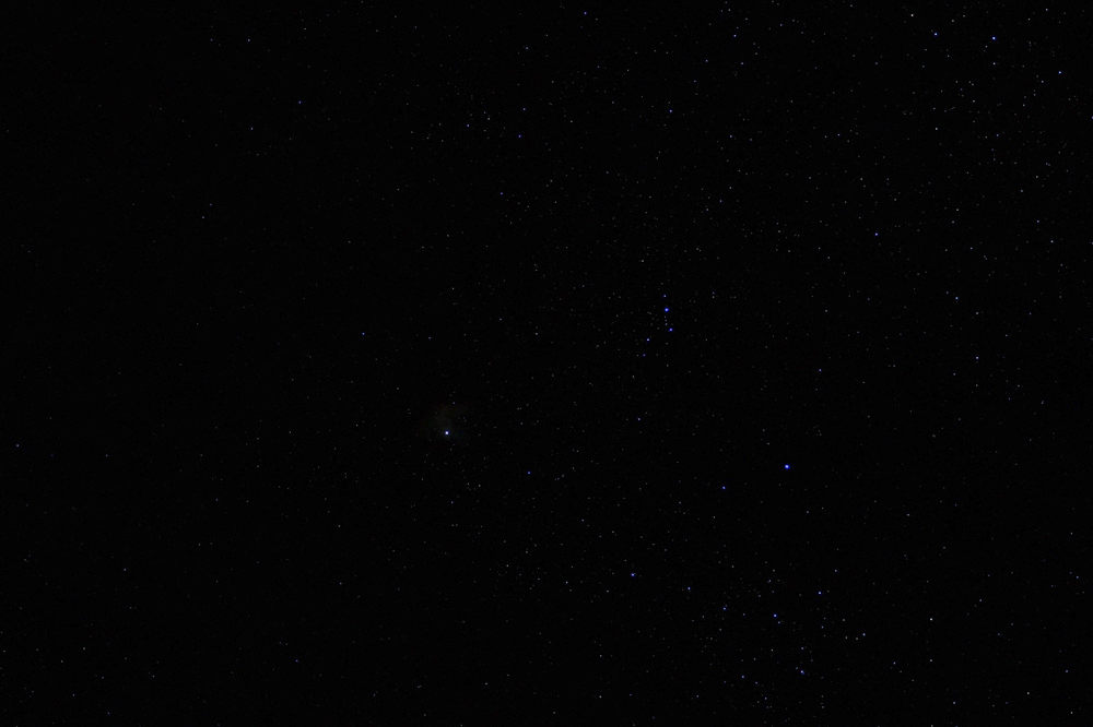
With some small breaks in the clouds visible I took a series of exposures before the clouds thickened. I could only see some stars in one of these frames as shown below.

I imported a jpeg of this image into Adobe Photoshop and used my usual method of removing light pollution, and in this case I hoped, the thin cloud. I now use a two stage process. In both stages, I duplicate the image to give two layers and apply the ‘Dust and Scratches’ filter to the top layer with a pixel size of 24 pixels. It thinks that the stars are dust and removes virtually all of their presence.

Some evidence of the bright star just left of centre remained which was cloned out from adjacent parts of the image and then a Gaussian Blur is applied with a radius of 15 pixels. What results is an image of the clouds/light pollution. In the first pass I set the blending mode to ‘Difference’ and flattened the two layers with an opacity of 50%. The evidence of the clouds/light pollution is reduced. In the second pass exactly the same process is undertaken, but this time with an opacity of 100%.
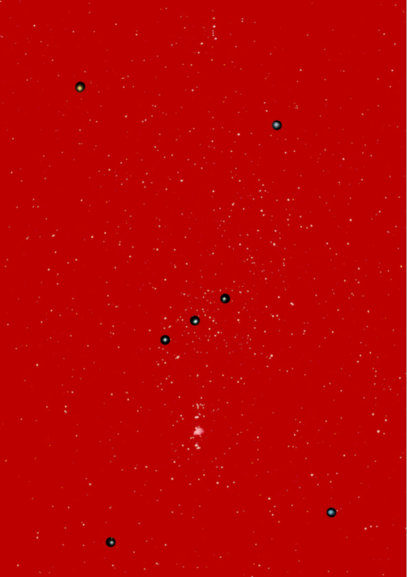
The light pollution and clouds have been removed – just a few stars are visible.
This image was ‘stretched’ by using the ‘Levels’ function with the centre slider set to 1.2 (moved over to the left ) and applied several times. This increases the brightness of the fainter stars more than the brighter ones. I was somewhat amazed at the number of stars visible in what was a single 30 second exposure.
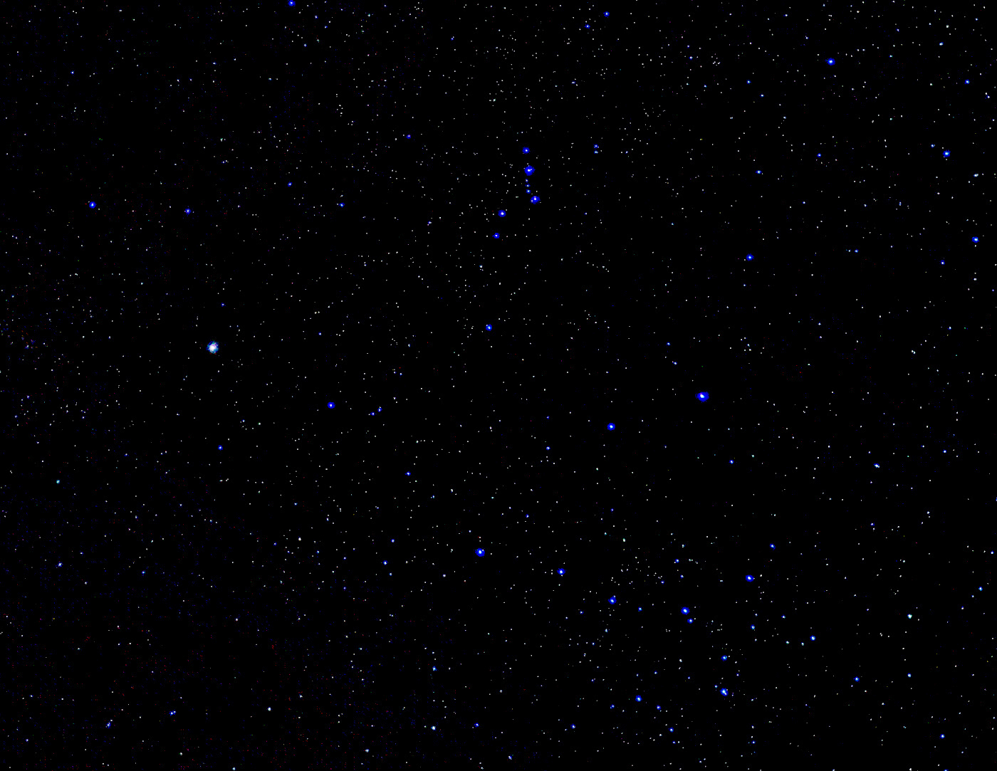 (On my computer screen, far more stars are visible)
Thoughts about Light Pollution
This image was taken about one mile from the centre of a town so light pollution would be expected. The above procedure removes it but it is still far better to observe or image from a dark sky. The light pollution will mask anything fainter than its brightness – faint stars, nebulae, dust clouds and galaxies for example. It does not matter how long the exposures are or how large the telescope aperture, they will be hidden from view.
One could image fainter stars by increasing the focal length of the lens. If, say, part of this region was imaged with a 110 mm focal length lens, only one quarter of the area of sky would be imaged, so only one quarter of the light pollution that covered the sensor when the 55 mm lens was used would fall on the sensor when the 110 mm lens was used. Its effective brightness is thus less and this would allow fainter stars – whose brightness, being point sources, is not reduced – to become visible. Sadly, extended sources, like nebulae or galaxies, will have their light spread out as well and their visibility will not be increased.
A Plate Solving Program
I should have known what stars were visible in the image, but as it was the first use of this APSC sensor and lens I was not sure of the image scale. So, not too sure what stars I had imaged, I submitted the image above to ‘Astrometry.net’ – a ‘plate solving’ program.
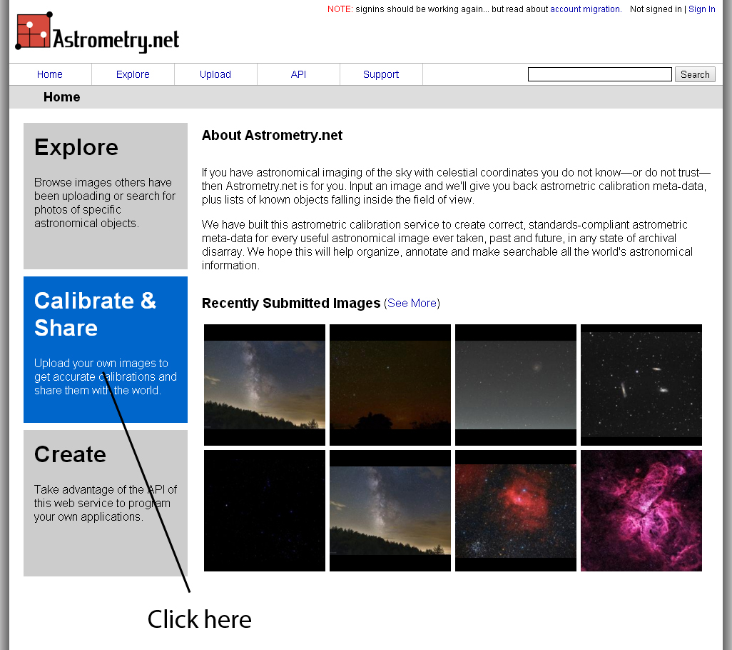
One is asked to select an image and then upload it.
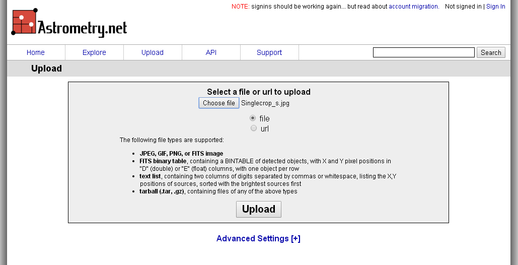
The submission was accepted.
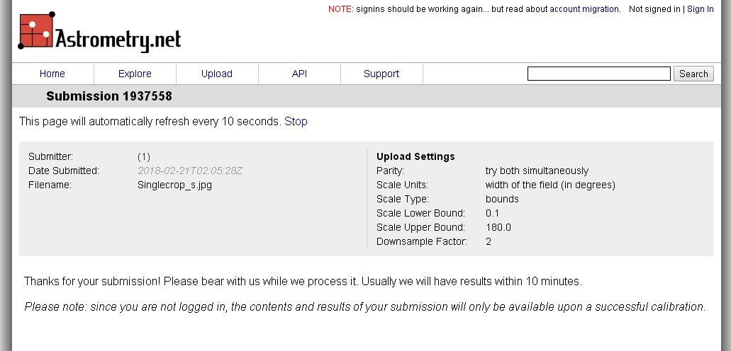
After some time this screen appears.
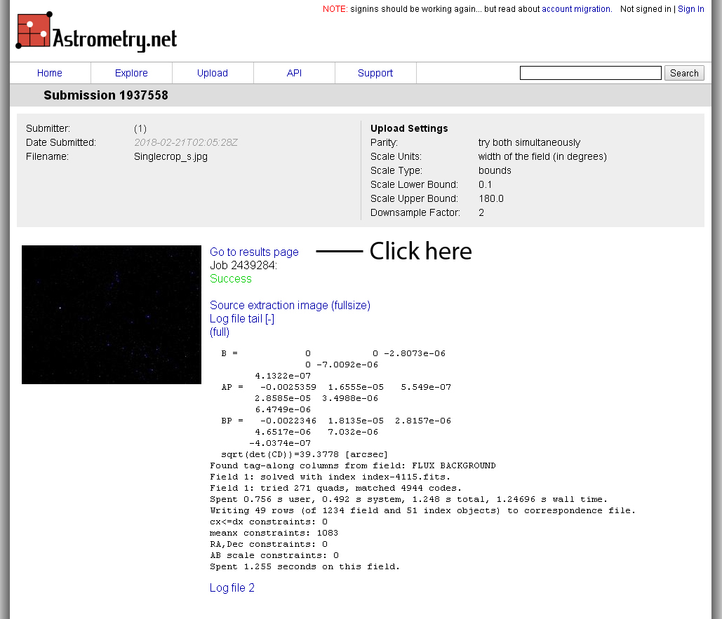
And one clicks on ‘Go to results page’. The result is very neat! This is a very nice piece of software.
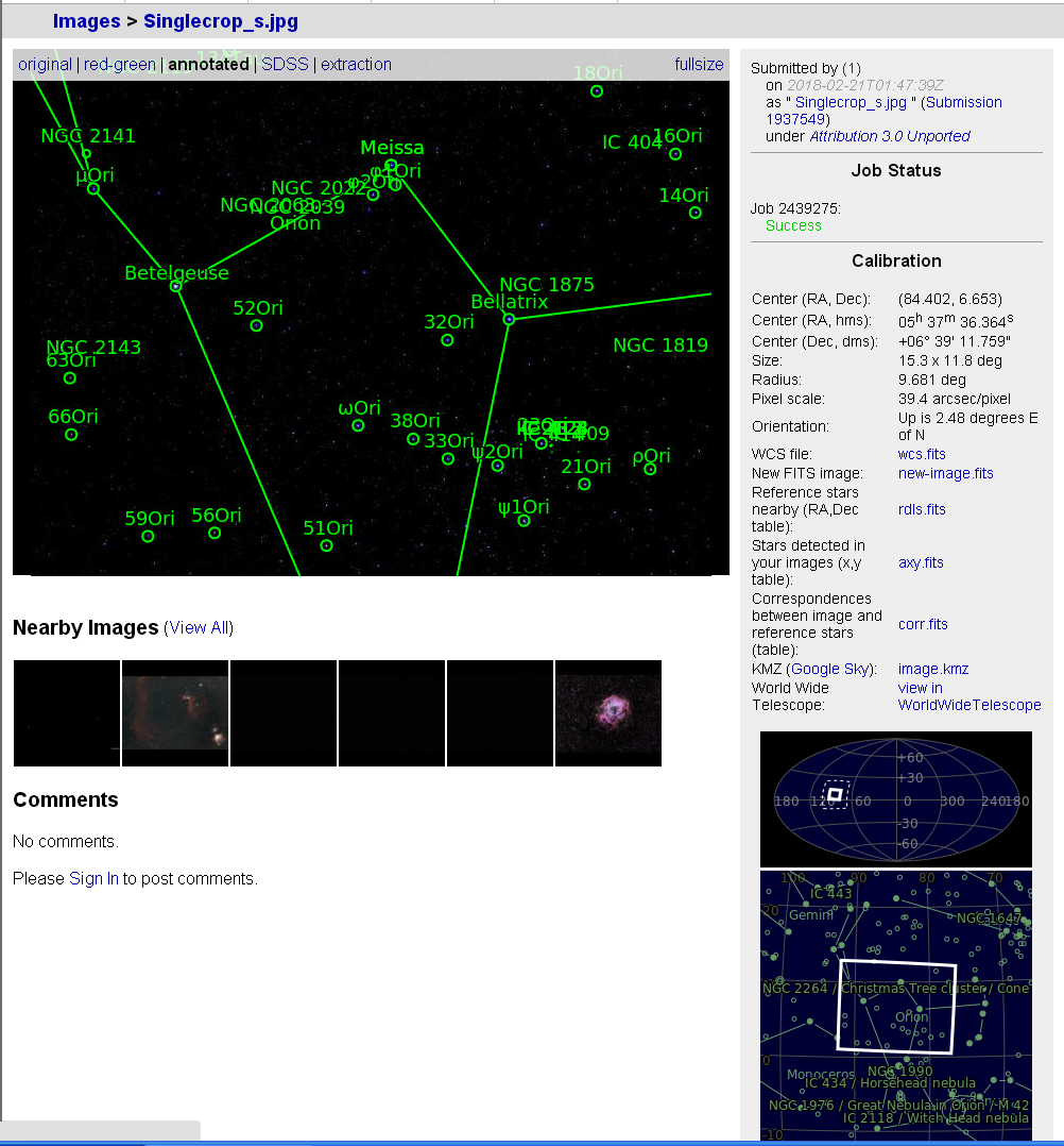
As shouId have been obvious, I was imaging the upper part of Orion. But it did mean that I had discovered a very useful program.
Imaging through fleeting clouds
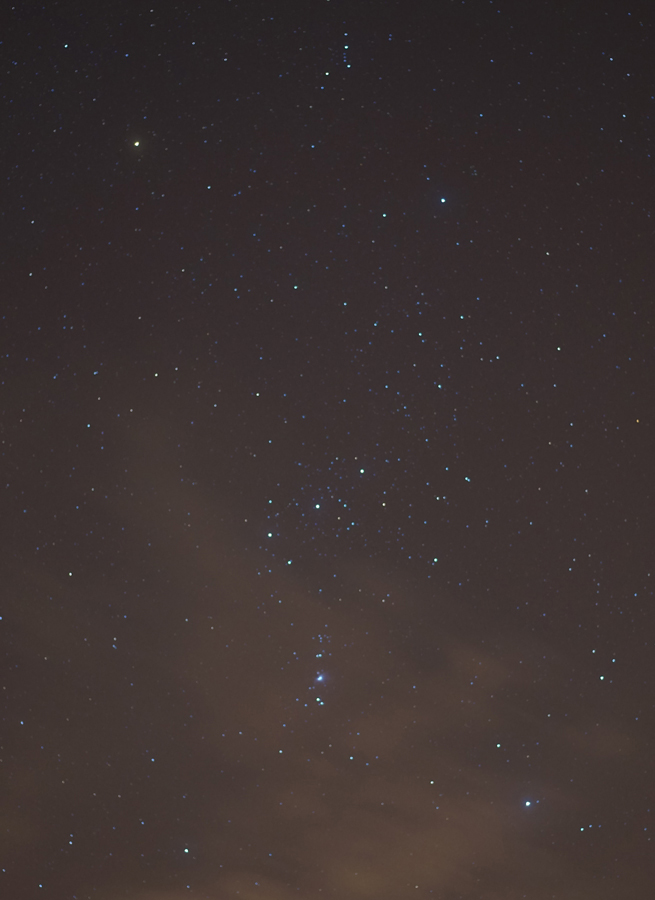
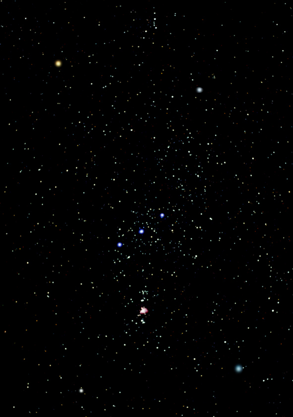
An hour later there were some more substantial breaks in the clouds, and, using the tilting screen of the camera, the brighter stars were visible so that I was able to align the sensor on the Orion constellation. The clouds were moving quickly across the sky so, at times, covering differing part of the image. This image shows one of the frames with partial cloud cover.
I was able to take 10 frames before total cloud cover resumed. At f/4 on an APSC sensor the 55 mm Nikkor lens would not give rise to any vignetting so no ‘flat’ frames were taken. Using its ‘Long Exposure Noise Reduction’ procedure, the camera follows the taking of each light frame with a second ‘dark’ frame with the same exposure time. This is subtracted, in camera, from the light frame so no individual dark frames needed to be taken. [In cold conditions, I would prefer not to use this noise reduction procedure as it halves the total imaging time and also adds some noise into each light frame but, in the A5000, this cannot be turned off.]
Deep Sky Stacker (DSS) seemed to have problems processing the Sony raw files so I converted them into .dng files using the free program Adobe Dng Converter. To remove the clouds from the image I used the ‘Median Kappa-Sigma’ stacking mode rather than the ‘Average’ mode. This looks at every pixel in all the frames and ignores those which differ by too much from the average (as when, as seen above, a cloud covers part of the frame). The effect is to remove their presence just as was desired.
The output from DSS then had the two pass light pollution action applied as described above before being was stretched using several applications of the ‘levels’ tool.
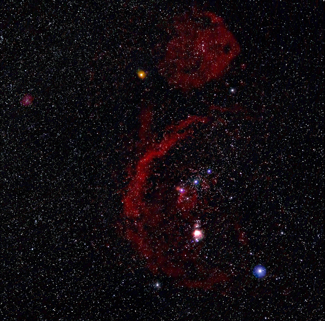
As usual, digital images of constellations do not look as good as those taken with film cameras as the latter, due to halation within the film, enlarges the diameter of the brighter stars making them stand out from the fainter ones. To simulate this effect the four corner and three belt stars were selected as seen in the mask below.
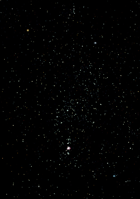
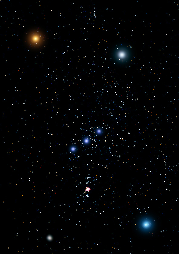
A Gaussian blur was then applied to expand them, but this also reduces their brightness. To bring the brightness back, the ‘Brightness/Contrast’ tool was applied. Standard sensors only record about one quarter of the H-alpha emission which should be seen in the Orion Nebula. To lift this in the nebula region, this was selected and in levels, the red channel brightness increased a little and a little Gaussian blur applied to smooth the region somewhat to give the final result below.
If you search for Orion images on the web, you will find some where the brightest stars have a ‘halo’ around them. These were, I suspect, made using film cameras with a ‘soft focus’ filter applied over the lens. A similar result can be produced by stretching a piece of black nylon stocking over the lens. The grid of fine strands has a similar diffraction effect. One can simulate this digitally (should one want to – and I am not sure about this) by selecting just the brightest stars, painting the rest of the image black and applying a Gaussian blur with a wide radius then bringing back the brightness somewhat. This results in a few diffuse regions at the positions of these stars. If the original image, above, is pasted over this image and the’Screen’ blending mode selected, the result shown below is produced when the two layers are flattened.
I have made far better Orion images (see below) under dark, clear skies, but I hope that this might serve to show you a couple of useful techniques and the result was actually quite pleasing – and it did show me that I had a useful lightweight imaging tool to take to the southern hemisphere. [On a warm night, due to the fact that then rear screen lifts to a vertical position a thin ice pack can be held by elastic bands against the rear of the camera – close to the sensor. This will reduce the increase in the sensor’s temperature as a continuous sequence of frames is taken and hence reduce the noise in the frames to be stacked.]
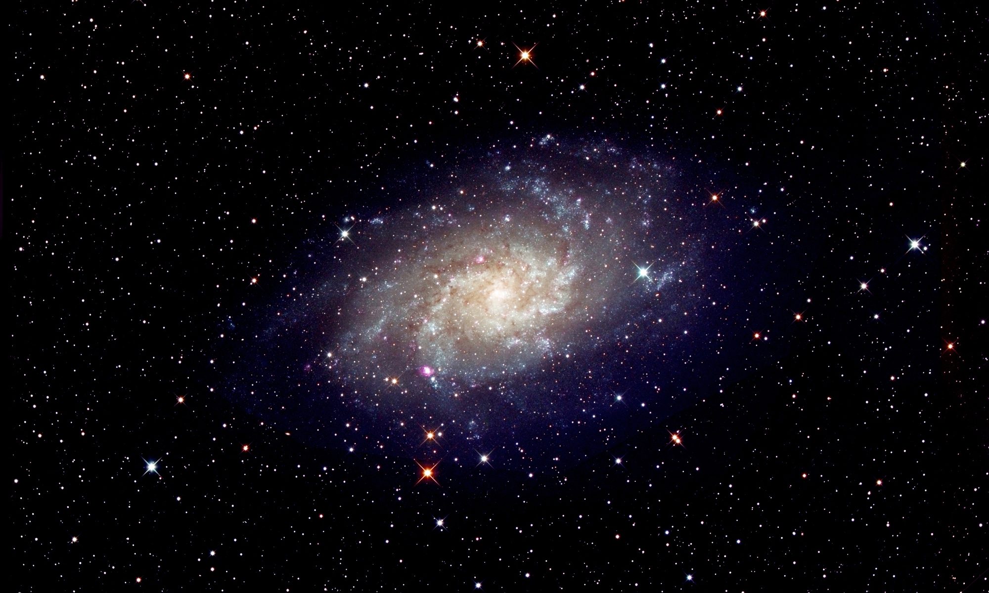
Orion imaged from New Zealand and the UK
This image is a composite of two images. The ‘RGB’ image was taken in New Zealand with the same system (Panasonic GX1 and 20 mm prime lens) as that used to take ‘A beautiful Southern Hemisphere Skyscape’ as described in the digest. The H-alpha image was taken in the UK using an SBIG, 8 megapixel, CCD camera and H-alpha filter using a prime Nikon 35 mm lens. The H-alpha image was scaled and aligned to the RGB image and the two blended together using the ‘Screen’ blending mode.