[This is just one of many articles in the author’s Astronomy Digest.]

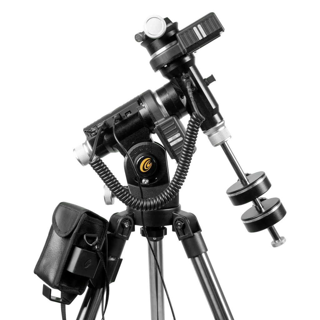
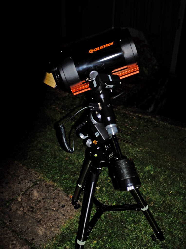
This relatively inexpensive  mount, costing ~£350, is an excellent small equatorial mount that could be used with an 80 mm refractor when used with the two supplied 1kg counterweights but, as described below given additional counter weights, it can support a 6 inch SCT or 127 mm Maksutov.  Used as such, it would make a very nice ‘get up and go’ telescope system to take out to dark sky locations.  There is no hand controller and the user’s Android or Apple tablet or a Windows 10 laptop is usually used to control the mount over WiFi using the, free to download, ‘Explore Stars’ App. 

The mount is provided with 2 (beautifully finished), 2.2 lb, counterweights, capable of balancing, for example, an 80 mm refractor.  For visual use the mount can handle a total weight of telescope plus counter weights of ~19 lbs for visual observing or ~15 lbs for photographic use.  However, dependant on the type of telescope to be used, additional counterweights may well be needed.   When at the furthest end of the counterweight arm, the two supplied weight’s centre of gravity is 11.5 inches from the axis of rotation.  This gives them a turning moment of 4.4 x 11.4  =  50 lb inches.   A refractor, when mounted, would have its centre of gravity some 7.5 inches from the axis of rotation so, when using the supplied counterweights, it weight could be up to 50 / 7.5  = 6.7 lbs.   In contrast,  a Celestron C6 Schmidt-Cassegrain with a weight of ~9 lbs including eyepiece and finder scope, has a centre of gravity some 9 inches from the axis of rotation so would have a turning moment of 81 lb inches.  It would thus need a counterweight of around 7.5 lbs. The 5 lb counter weight that I combined with one of the two supplied 2.2 lb counter weights has a turning moment of 7.2 x 11 = 79 lb inches and this worked well.  (A slight imbalance helps prevent backlash in the worm drive.)  This gives a combined weight of ~16 lbs, well within the mount’s nominal weight allowance.  A 6 inch Celestron Schmidt-Cassegrain or a 127mm Macsutov would thus make a very suitable combination providing an additional ~3 lbs of counterweight is added.  These two telescope types being ‘short and fat’ have a lower moment of inertia than long refractor tubes or Newtonians making it easier for the mount to control their movement.  [Telescope House sell the 1kg Explore Scientific counter weight for £21.50.  One might just be sufficient thought the combined weight would be a little low at 6.6 lbs.  A second additional weight would allow for a perfect balance.] 

I have recently bought one for use largely as an astrophotography mount for use with my longer focal length lenses and small refractors but also with a Celestron 6 inch Schmidt-Cassegrain telescope for use at our astronomy society’s star parties. 

I purchased it as I was impressed by two aspects of the mount’s design; firstly that the worms used for the RA and Dec drives are belt driven which should give quieter slewing and smother and better tracking than those mounts which are gear driven.

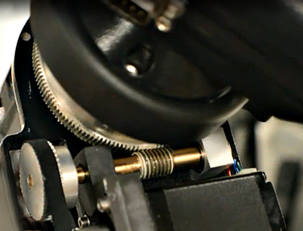
The RA gear has a diameter of ~ 7cm, which is twice that of the typical star tracker, so, in combination with the belt drive, the tracking should be both more accurate and smoother than a typical tracker so making it an excellent mount for use with a small refractor for astroimaging.

Secondly the two axes are equipped with variable tension clutches as used on my £3,000 Losmandy GM8.  This is very useful when manually moving to an area of sky for wide field imaging as, with the correct tension applied, the camera’s field of view can be easily selected and the mount will stay in position without further adjustment as it starts tracking at a sidereal rate.  When slewing, the mount quietly ‘sings’ at quite a high pitch, indicating  a very precise stepper motor drive and then, whilst tracking, is essentially silent.

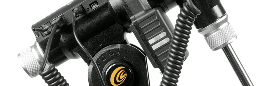
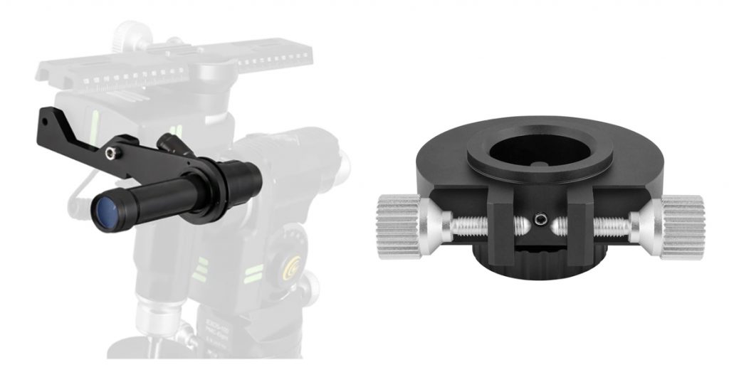
A battery pack to contain 8 C batteries is supplied to power the mount and can be secured in a bracket on one of the tripod legs if an external 12 volt battery (such as Celestron ‘Power Tank’) or AC adapter is not used.   Thoughtfully, ‘glow-in-the-dark’ markings are placed on the mount and tripod to avoid tripping over them under very dark skies.  As supplied, there is no fine adjustment to set the azimuth of the mount to align on the North Celestial Pole.  I have not found this to be a problem but, if desired, an ‘Azimuth Adjuster Adapter’ can be purchased.

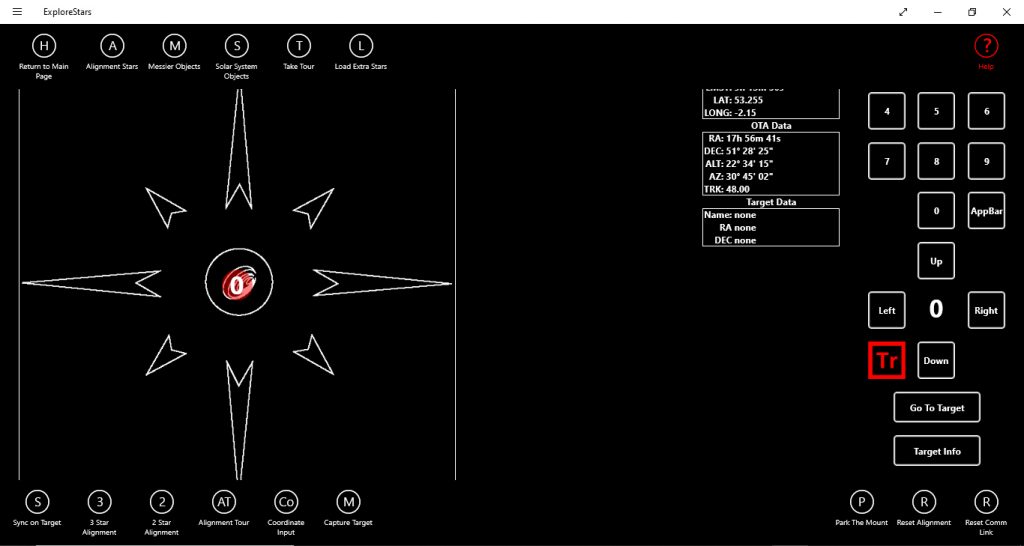
As my Android tablet is too old to accept the ‘Explore Stars’ app, I am using an i5 laptop to control the mount.  There can be problem with the latest Window’s 10 versions in that it may not immediately connect to the mount’s WiFi channel but there is a ‘work around’ documented by Explore Scientific.

I have found the App to be very nice in use with, in daylight mode, colour images along with descriptions of many of the objects in its very extensive catalogue.  If desired, one can switch it to a red ‘night time’ mode.  Having levelled the, quite solid, 1.25 inch tube, tripod using the built in bubble level, the mount is aligned on the North Pole using a sighting tube through the RA axis, though a polar telescope is available as an accessory.  I have made an adapter so that I can use a laser pointer projecting its beam through the sighting tube to give a fairly accurate alignment of the North celestial Pole, though I could also arrange to fit my QHY PoleMaster on the mount for more precise alignment. Before powering up the mount the telescope should be set in the ‘Polar Home Position’ with the scope aligned on the Pole.

Given the site co-ordinates (the app will use the time in the tablet or laptop) either a two or three star alignment procedure is carried out with the mount providing suitable stars to align on. 

For each star, fine adjustments are made to centre the star as necessary using adjustable slew rates in RA and Dec.  I like the fact that, each time, the selected star is shown on a simple star chart display so one can be sure one is centring on the correct star in a constellation. 

It is also possible to do a ‘1 Object’ alignment’. From the ‘Polar Home Position’, one could (as in the early evening in October 2020) simply select Jupiter and slew to and align on that very obvious target! Then, from the App Commands, select ‘Sync on Target’ and this will have made a single alignment setup. Depending how well the mount is levelled and aligned on the Pole, this may well be sufficient but, of course, a ‘3 Star Alignment’ will give better ‘GoTo’ performance across the sky.

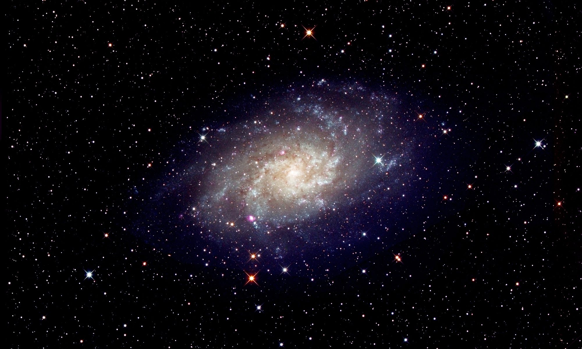
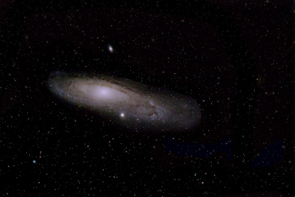
On another night I wanted to make a ‘test’ image of M31, the Andromeda Galaxy, so I selected Mars – a very obvious target, also in the east – and, having aligned the mount, simply slewed and centred it is the field of view of my full frame Sony A7S camera. Then in the Apps commands, I synchronised onto the target. This should mean, that in the eastern part of the sky the ‘goto’ ability should be fine. So it was as when I slewed to M31 and took a short exposure, it lay near the centre of the field. In fact, the heart of the galaxy, looking like a faint star, was just visible in the camera’s live view so I could easily centre it in the frame using the slewing controls. The mount then tracked accurately across the sky as short exposures were taken so as not to overexpose the centre of the galaxy.

On the other hand, should I wish to use the mount with my Celestron C6 at a star party and view a selection of objects, it would be well worth using the 2 or 3 star alignment method.

Having completed the alignment, one can, as one would expect, choose from objects within the catalogues that lie above the horizon and the mount will drive to their position and then track them at a suitable rate across the sky.  The Explore Stars App provides images and descriptions of many of the most popular objects such as those in the the Solar System or Messier catalogue.

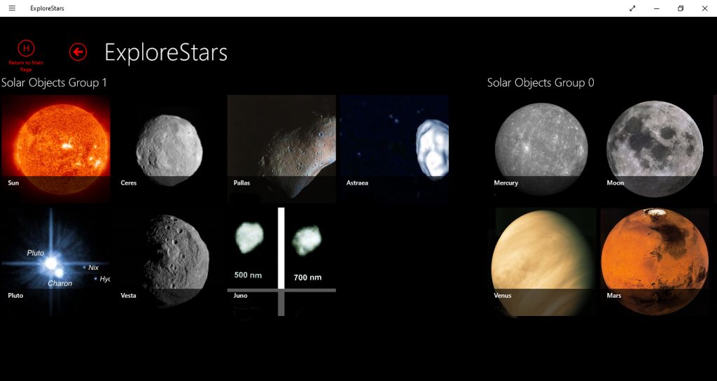
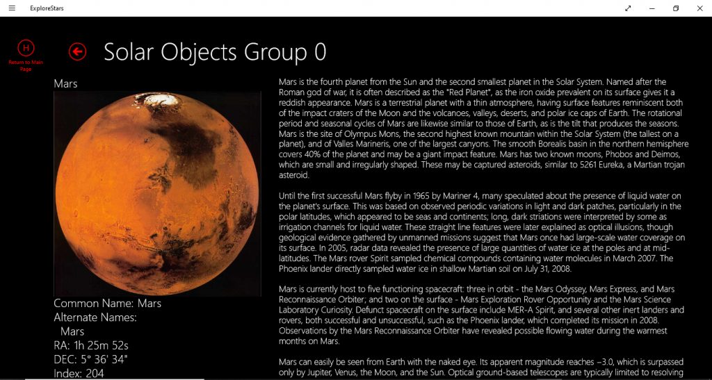
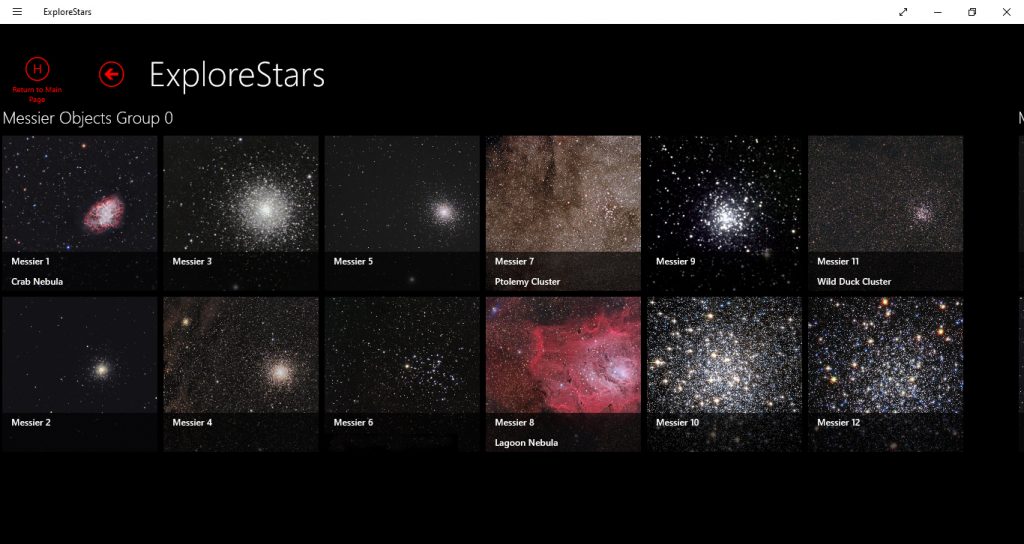
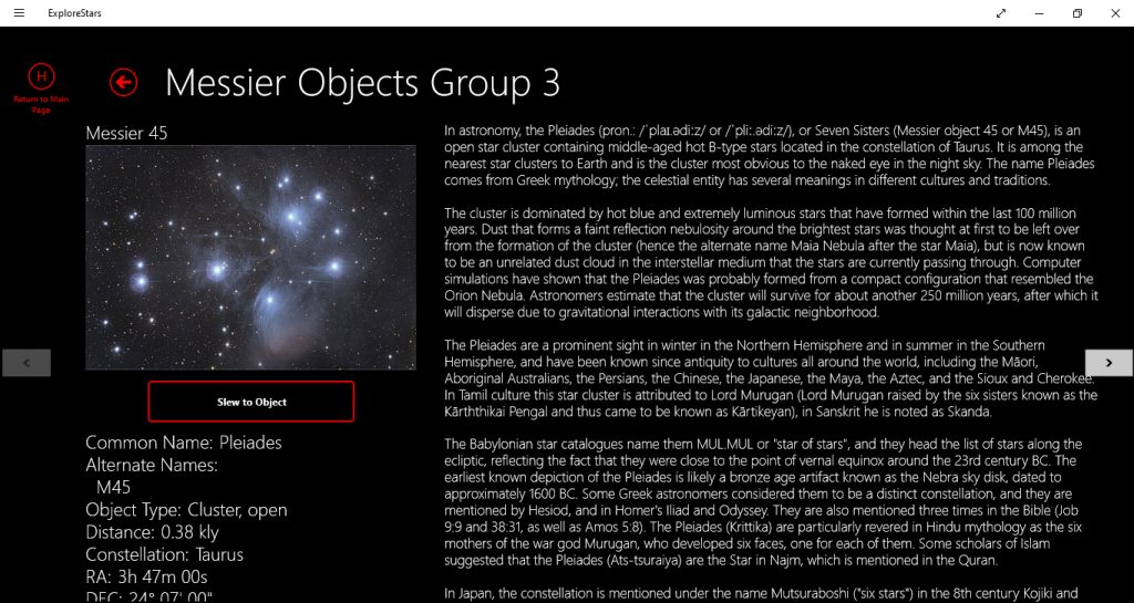
For accessing any of these Solar System or Messier objects one can also use the ‘Search’ Command (perhaps slightly quicker) as well as any of the other objects in the extensive database including the NGC and IC objects.

Though I suspect the majority of users will use the Explore Stars App.  Details are given on their website and on YouTube videos to enable one to download the ASCOM software interface so that the mount can be controlled by planetarium software such as Stellarium.

In the early versions of the mount, it would stop tracking if the WiFi connection was lost. I believe that the latest mounts, or with the updated software that can be installed into the mount, this does not happen and the mount will keep tracking usually at sidereal rate. I have not bothered to update the firmware as, with my laptop, I have never lost contact.

One final point.  There is a very good user group and I have been very impressed how Jerry Hubbell (what an appropriate surname), Explore Scientific Vice President Engineering, along with Wes Macdonald have been very helpful to any users of the mount who have problems.

First Light Images

This was the ‘first light’ image using the mount of the region around Deneb and was captured using a Sony A7S full frame camera and Teleskop Service 65 mm, 422 mm focal length, quadruplet astrograph.  A total of 50, 30 second exposure, frames were aligned and stacked in Sequator.  I am sure that longer exposures can be used, but the Sony camera suffers from the ‘Sony Star Eater’ problem with exposures over 30 seconds long.

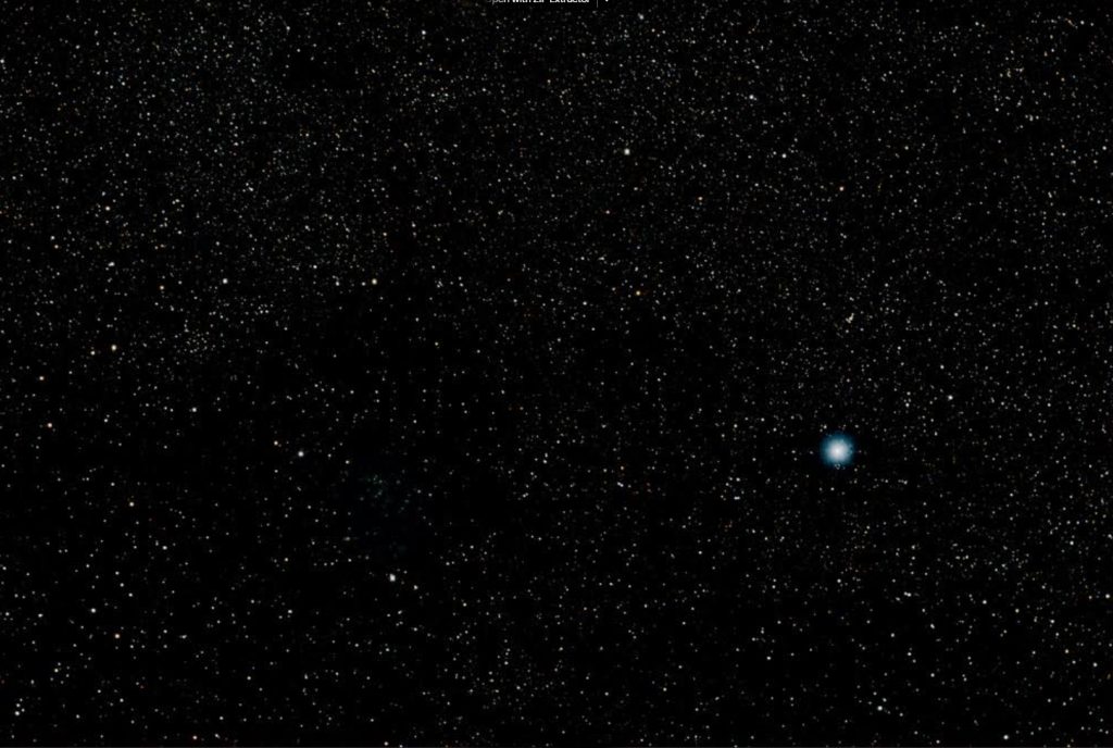
The second image is a composite of two images taken with the same camera but attached to a Takahashi FS60, 354 mm focal length, telescope.  This time, the exposure was just 15 seconds – not to avoid tracking problems but so as not to over expose the heart of the Orion Nebula.  This is shown well with the ‘Running Man’ nebula just above and also, just to the left of Alnitak, the lower of the belt stars, the ‘Flame Nebula’. The humidity in the atmosphere when this image was taken has given a diffuse glow around the brighter stars.

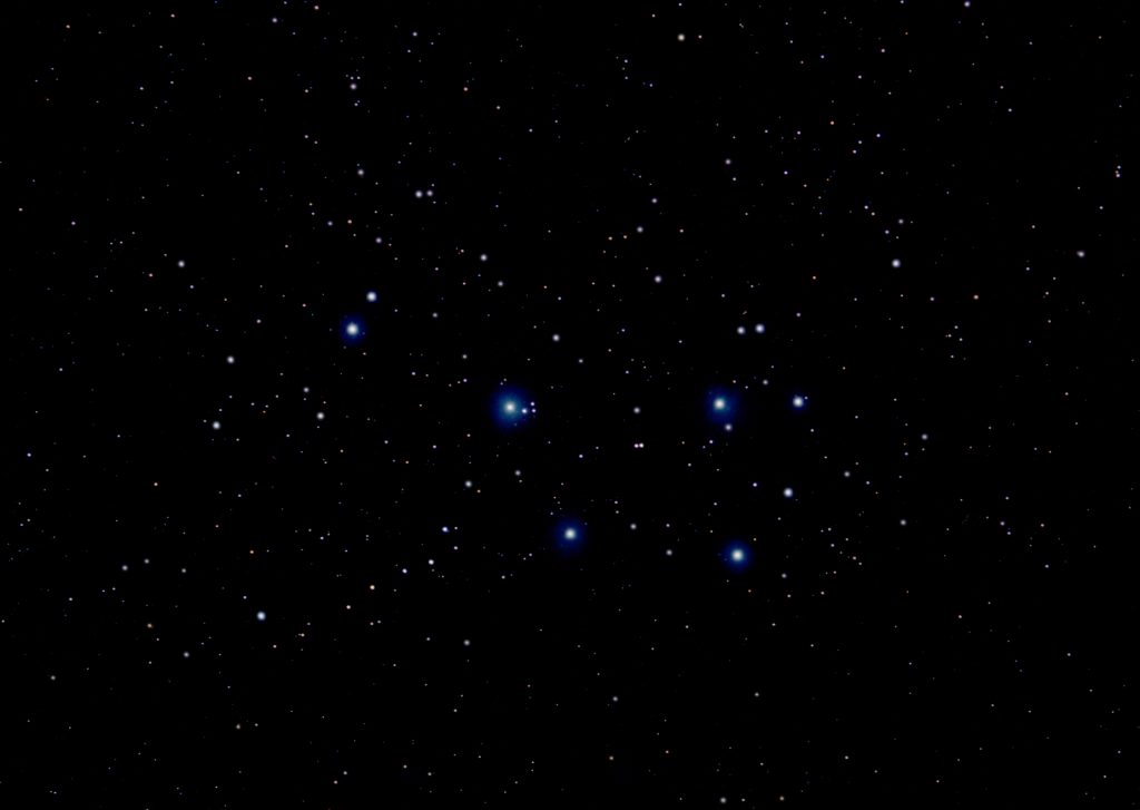
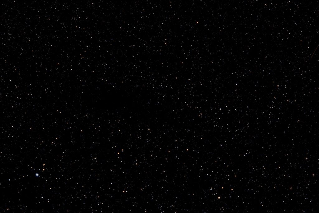
The following image is a 96 second total exposure image of M45, the Pleiades Open Cluster, made up just 6, 16 second exposures taken before clouds rolled in. An 80 mm aperture, 500 mm focal length, semi-apo refractor was used with Teleskop Service 2 inch Field Flattener and Sony A7 II full frame camera. With just a short total exposure, one could not expect to see any of the beautiful nebulosity, but I include it to show the quality of the stellar images that can be achieved using the mount.

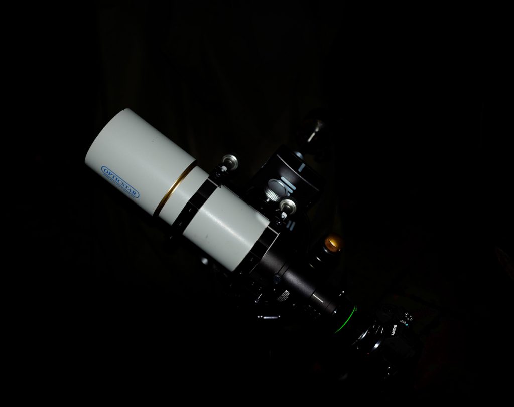
An Imaging example using an 80 mm refractor

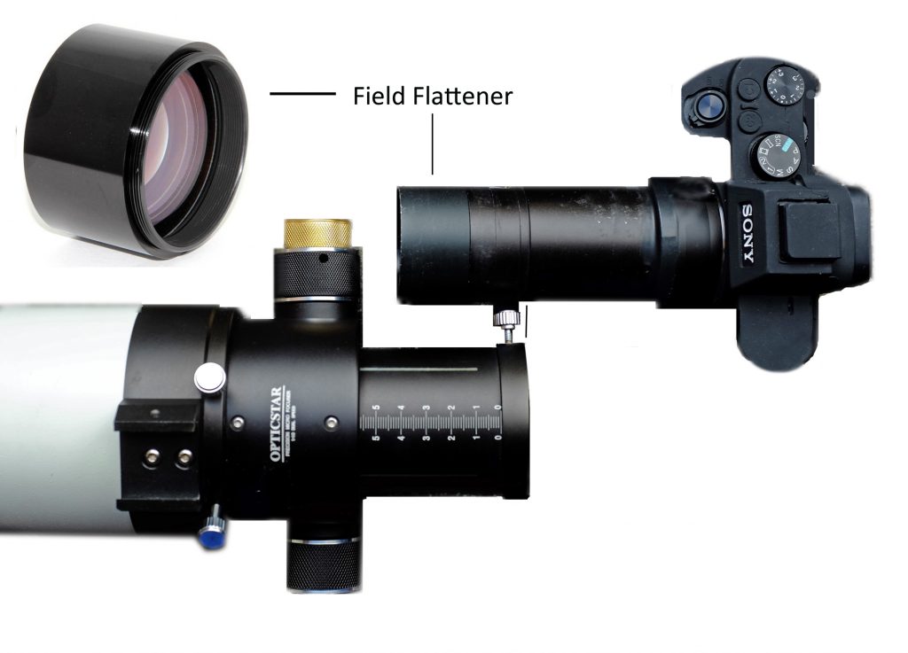
The iEXOS-100 makes an excellent star tracker easily able to support an 80 mm refractor such as my semi-apo,  FPL-53 doublet, telescope having a relatively short focal ratio of f/6.3.  It is very well corrected for chromatic aberration showing essentially no false colour around stars.  It was coupled with a Teleskop Service 2 inch field flattener with the combination able to cover a full frame sensor such as that in my Sony A7S, 12 megapixel, camera with little vignetting towards the corners.

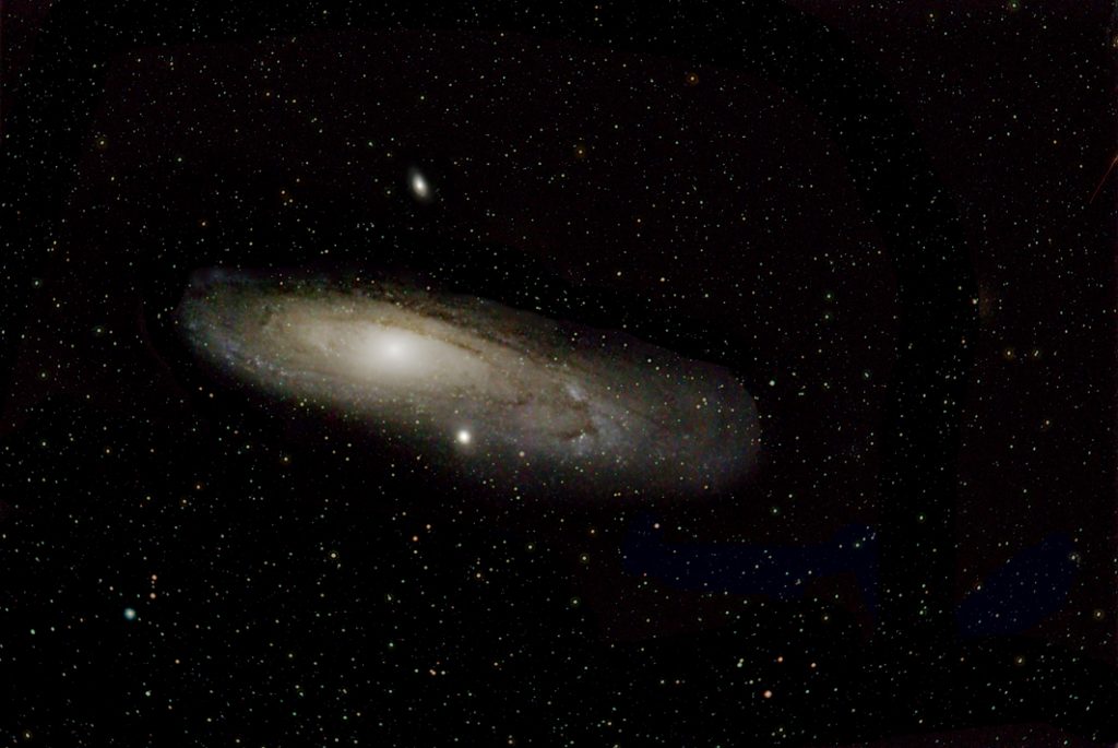
The final image, shown at the end of the article, is nothing special but it does show what this mount/telescope/camera combination can do under non ideal conditions and offers the prospect of making an excellent image when, after ‘lockdown’ in the UK, we are able to travel again to a dark sky location.

The field flattener has to be located ~12 cm away from the sensor which greatly helps its performance compared to typical flatteners which are located ~5.5 cm from the sensor.  In fact, the rear element of the flattener is some 3 cm within the telescope focuser barrel. This does, however, cause a problem. With a typical 6 inch dovetail bar, balance about the mount’s declination axis cannot be achieved and so a longer dovetail bar is required.

The Sony A7S live view is sensitive enough to show star fields and ‘focus peaking’ allows accurate focus to be achieved easily.  As precise focus is achieved very faint stars across the field come in and out of view as their light is focussed on fewer pixels.

The image was taken from a garden just 1 mile from a town centre so light pollution was expected as seen in the image produced by aligning and stacking the frames in Sequator (see article in the digest).  The total exposure was 40 minutes.

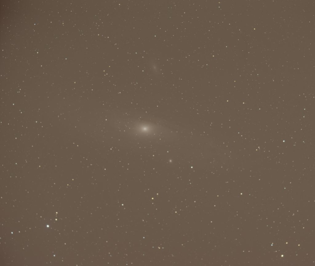
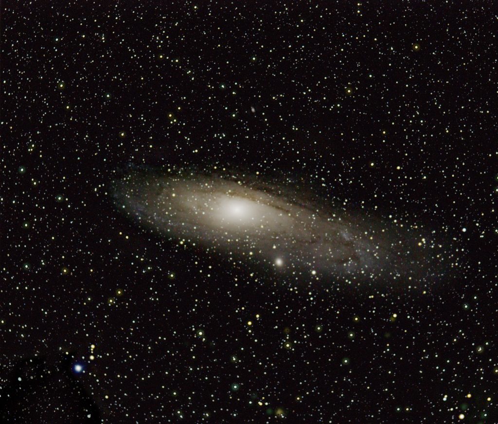
As M31 was at a high elevation, one might hope that the level of light pollution would be constant across the field of view.  However, the minor vignetting will cause its effect to vary away from the centre of the field and so some care is needed to remove it.  The image, shown above, was duplicated and the ‘Dust and Scratches’ filter with a radius of ~15 pixels used to remove the stars.  Assuming that the light pollution will be constant in the region of the galaxy, the paint brush was used to sample its brightness and colour close to the galaxy and the galaxy region, including M110 above, ‘painted’ with this colour.  The two layers were then flattened using the ‘Difference’ blending mode.  The result was then stretched using several applications of a curve which lifts up the fainter parts of the image.

This image could be worked upon directly but it is better to separate the stars and galaxy and work on them independently.  The program Starnet++ was used to remove the stars from the image as described in the digest article ‘Using Starnet++ to enhance Nebula images’.

This is saved as ‘galaxy’, the original image is brought back and pasted over the galaxy image and the two layers flattened using the ‘Difference’ blending mode.  This leaves just the ‘stars’ in the image.   If desired, the star sizes could be reduced using the ‘Minimise’ filter. 

The galaxy image can be enhanced by applying some local contrast enhancement (*) and the saturation increased slightly to give the following image . [* By using the ‘Unsharp Mask’ filter with a large radius and small amount.]

The ‘stars’ image is then pasted on top and the two layers flattened using either the ‘Screen’ or ‘Lighten’ blending mode.   It is interesting that, using the opacity slider, it is possible to make the stars less apparent in the image so helping to showcase the galaxy. 

I then used a program called Siril to apply a ‘Photometric Colour Calibration’ to the image as described in the digest article ‘Using Starnet++ to help enhance Nebula images’. This gave a very pleasing result in terms of it colour balance as seen below.

Note: I purposely slightly miss-align the mount on the North Celestial Pole so that the captured image frames move very slowly across the camera sensor during the 40 minutes of total exposure taken for this image. The movement in each exposure was just 1.3 pixels, (so no star trailing was present) with a total movement across the sensor of 103 pixels. This reduces the effects of any hot pixels (no long exposure noise reduction was employed which halves the time capturing photons) and, perhaps surprisingly, no evidence of hot pixels was see in the stretched image – though it was a cold night. In addition, what Tony Hallas calls ‘Color Mottling’ (he is American) due to variations in the sensitivity of the different coloured pixels across the sensor is removed. [When autoguiding is used, ‘dithering’ is employed to achieve this, but this technique gives much the same result without autoguiding.]

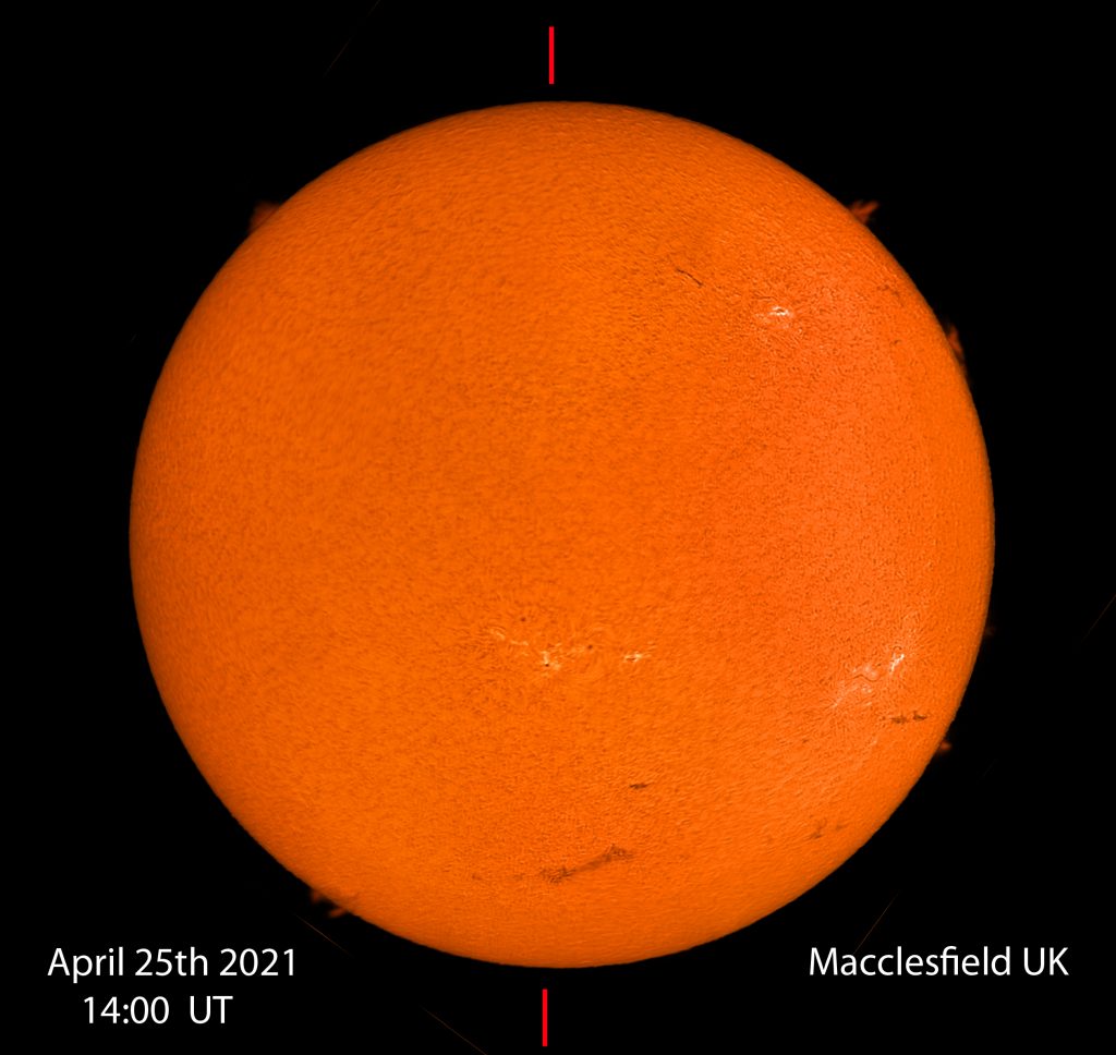
Imaging the Sun with a Solar Telescope and webcam

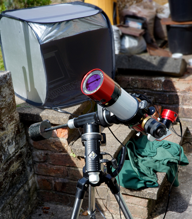
Obviously, one cannot align the mount on the North Celestial Pole in daytime but this is not a problem.  The important thing is to make sure that the mount is level with the latitude having previously been set correctly whilst observing at night.  With the bolt that holds the equatorial head to the tripod very slightly loose, and using a compass one should set the mount aligned as close to North as one can.  [At present in the UK a compass points very close to true north.] One then simply slews to the Sun.  One would not expect that it will be centred in the solar finder.  However, the only problem should be the inexact alignment North.  Simply rotating the equatorial head should then bring the Sun into view and the mounting bolt tightened.  Using the slew controls one can then centre the Sun in the finder and its image should appear on the webcam’s capture screen.  The mount was controlled using WiFi from an i5 laptop (seen within the hood) using an external SSD drive to store the captured video sequences.  

Having been in the doldrums for a couple of years now, the Sun’s surface is now beginning to become more interesting as the image shows.  It was taken with a Lunt Double Stacked 60 mm H-alpha solar telescope using a ZWO ASI 178 webcam whose exposure and gain was controlled by and the frames captured using SharpCap.  This was the first time I have observed a webcam’s output displayed on a screen and I could see the smoothness of the tracking – excellent – and the low periodic error as the Sun’s image slowly moved back and forth (in Right Ascension) within the frame.

A 2,000 frames .AVI sequence was aligned and stacked in Autostakkert! and the result processed and coloured in Adobe Photoshop.