APRIL 2018
An Imaging exercise – Bode’s Galaxy, M81 and the ‘Cigar Galaxy’, M82
An article in the author’s Astronomy Digest – https://www.ianmorison.com
This is a complete ‘walk through’ of an imaging exercise which I hope may provide some useful tips and advice − in particular as to how one can extract best the possible final image from the captured data.
Though I have been imaging for quite a few years now, I have never tried to image M81 and M82 (which lie at a distance of 12,000,000 light years in the constellation Ursa Major) and decided that I should give them a try. This example explains how I attempted to go about it and what I have learnt from my first efforts.
Choice of Imaging System.
This involves the choice of telescope and camera system. The first requirement is to choose a telescope which, coupled with an appropriate camera, will give the desired field of view. The program which helps in making the choice is the Astronomy.tools ‘Field of View Calculator’. One simply chooses a telescope from a very wide range listed (or specify a ‘custom’ scope) and camera (from both DSLR’s and CCD types – if yours is not listed give one with the same sensor size) and enters the name of the object to be imaged. The program then brings up a plot showing the field of view surrounding the object.
It does help to have a number of telescopes of differing focal lengths so that one can find the best match. Perhaps an imager might have one short focal length refractor, say 80 mm, f/6, ideal for wide field objects such as the Pleiades Cluster or the Sword of Orion, a telescope with a focal length of ~8-900 mm, probably a refractor, which would be ideal for galaxy clusters such as the Leo Triplet or, in this case, M81 and M82, and then a longer focal length telescope such as an 8-inch Celestron Edge HD Schmidt-Cassegrain or Vixen VC200L – both of which are ‘astrographs’ giving a smaller but well corrected field − ideal for globular clusters or planetary nebulae.
The choice will depend on the size of the imaging sensor; most DSLRs and quite a number of CCD cameras have sensors of APS-C size which can be used with most telescopes. Full frame (36 x 24 mm) sensors in DSLRs and CCD cameras will need to be used with astrographs that can cover them without too much vignetting.
I chose to use a 127 mm aperture, f/7, telescope to image the two galaxies in one field of view along with a ‘one shot colour’ CCD camera, the QHY QHY8L having an APS-C sized sensor. As the images were to be taken on what had been some of the warmest April days for 70 years, the fact that it can be cooled was quite important. The image below from AstroTools shows that both would be comfortably encompassed with this combination.
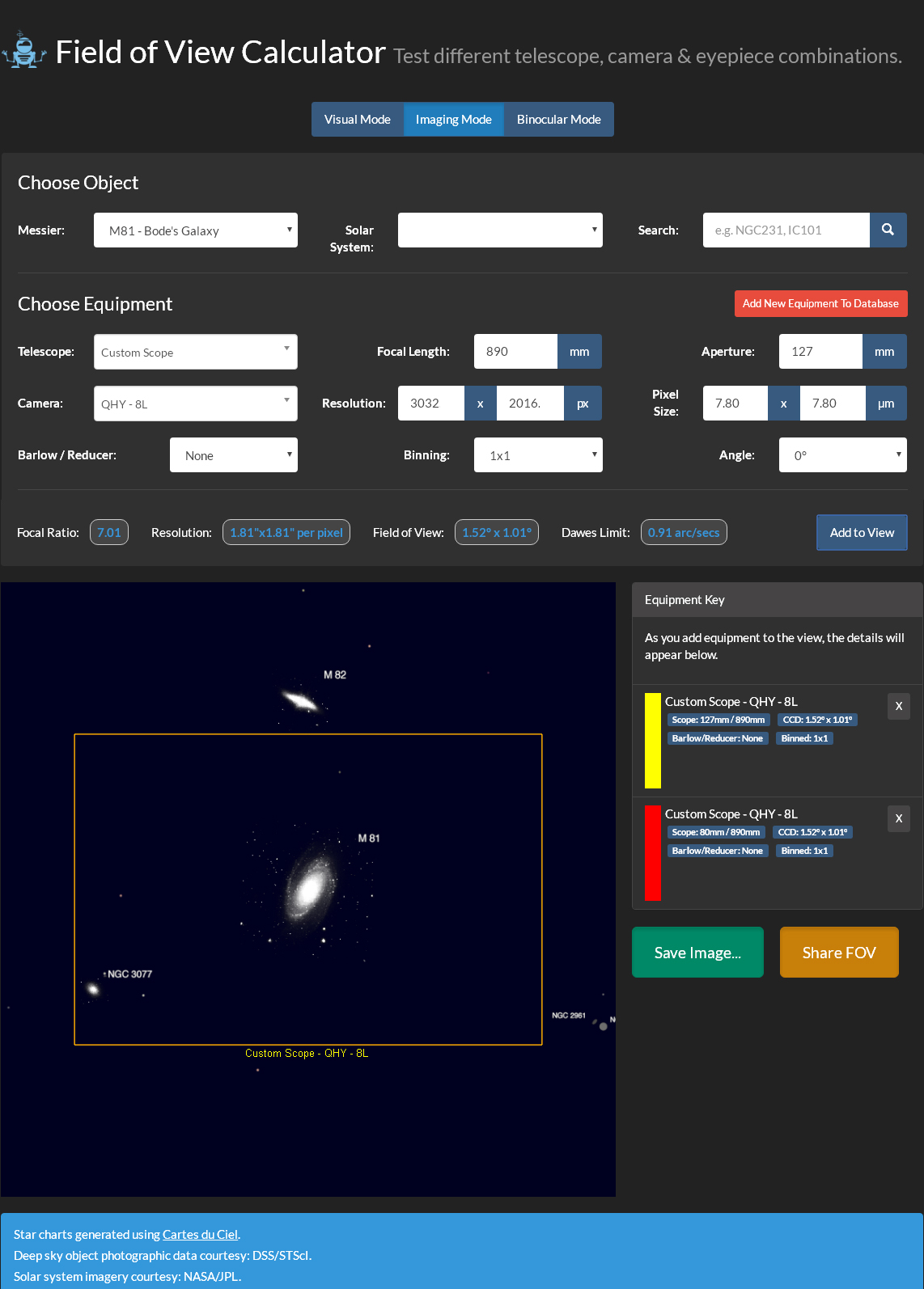
Astronomy.tools Field of View Calculator screen for my telescope and camera.
When searching for faint galaxies it helps if a go-to mount is well aligned and I used my QHY PoleMaster (see article in the Digest) to align it when Polaris became visible. I also first checked and then adjusted the time in its controller as it tends to run a little slow – an incorrect time will cause the mount’s pointing to be off in right ascension.
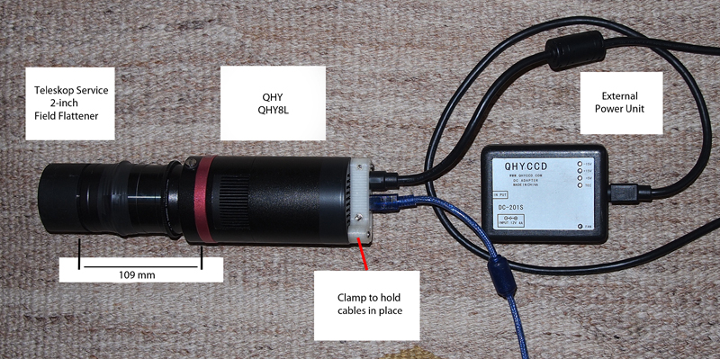
My 127 mm, f/7, refractor is not an astrograph it will suffer from field curvature so that stars near the corners of the field of view will be out of focus and may be distorted. To correct for this I have a Teleskop Service 2-inch Universal Field Flattener which can be used for refractors of focal ratios from f/5 to f/8. [It can be bought for ~£180 from 365 Astronomy.] The rear of its lens mount has to be at a distance of 109 mm from the sensor of the camera so I made a suitable length adaptor on which to mount the QHY8L.
There is a further advantage of having a lens element prior to the CCD camera so, if not using a field flattener or flattener/reducer, I would mount a clear filter at the outer end of the 2-inch barrel which locates within the telescope focuser. In either case, this reduces the amount of air in contact with the cold aperture of the camera and so reduces the risk of any condensation forming upon it. [This is most important if an open tube telescope is used.]
The QHY8L employs a Sony ICX413AQ CCD sensor with 6 million, 7.8 micron, pixels covering an area of 23.4 x 15.6 mm. It was once used in the Nikon D50. It has a slim round body so is very suitable for ‘hyperstar’ systems but, to achieve this, has a separate small power supply unit requiring a 12 volt input. It can be cooled to around 40 Celsius below ambient temperature. It is now supplied with a 3D printed clamp to securely hold the USB2 and power cable to the back of the camera. [The square USB2 cables are notoriously insecure.] 2×2, 3×3 and 4×4 monochrome binning modes are available to give greater sensitivity and so help in finding and aligning on faint objects – such as these galaxies – with short exposures before switching to the un-binned colour mode.
Capturing the imaging data
My imaging attempts was on the 18th and 20th April 2018. On both nights a crescent Moon hung in the western sky and so, before it became dark enough to check the mount’s alignment, I imaged it in the infrared using a Point Grey Chameleon webcam.
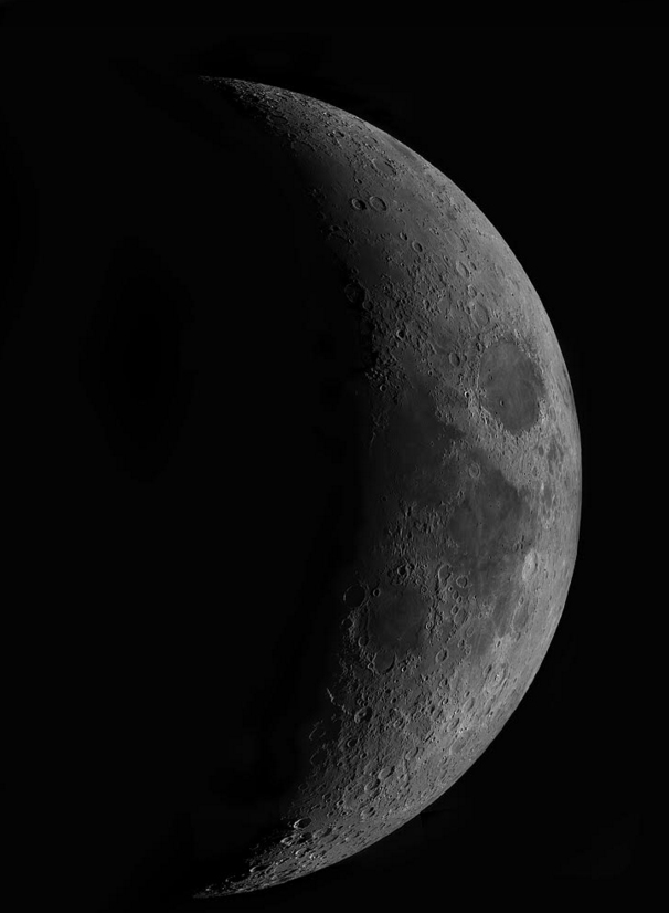 Moon April 20th 2018
As this was a new telescope/camera combination I had no idea where the correct focal point would be so I first slewed the telescope to Arcturus, quite high in the east. This made it quite easy to focus the camera as, even when way out of focus, the star could be seen as a large spherical disk. The indication that fine focus has been achieved is when many faint stars appear in the image.
Sensor Cooling
The advantage of using a QHY8L over the Nikon D50 whose sensor it shares is, of course, the fact that it can be cooled and so significantly reduce the dark current and its inherent noise. Dark current reduces by about one half for every 6 degree reduction in temperature. The sensor in a D50 would probably stabilize at ~12 Celsius above ambient temperature, say 20 Celsius, so with a sensor temperature of -24 Celsius this is a difference of 44 degrees giving a reduction in dark current of ~128 times and that of its noise by the square root of 128, that is ~11 times. Good.
Within the EZCAP screen, the temperature control window can be opened and the temperature can be set either to a defined temperature or a fixed power ratio. The percentage Peltier cooling power employed is indicated in the control window, and I would not really want the continuous power used to be greater than ~50% (shown in the window) to avoid stressing the system so I simply set this to 50% and was somewhat surprised that the sensor temperature stabilized at -27 Celsius.
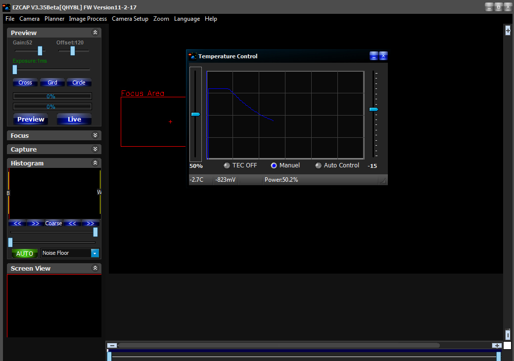 EZCAP temperature control window as the temperature falls to a stable value
I then slewed to M82 with the EZCap camera capture program set to ‘preview’. This uses the 4×4 binning mode for the highest sensitivity and takes continuous frames with exposures of up to 10 seconds. Pleasingly, the two galaxies were visible in the field of view and the telescope’s pointing was adjusted so that both were suitably framed in the image.
The camera was then switched to the ‘capture’ mode and, to obtain a colour image, the binning mode was set to 1 (meaning no binning). Some trial captures with an exposure of 25 seconds were made in which the two galaxies could be seen with even a hint of colour showing in M82. The ‘planning screen’ was then opened up and the program was set to capture 100 frames giving a total exposure time of 41 minutes. The data was processed as described below but it was obvious that the total exposure was not really long enough. I thus imaged the two galaxies two nights later following the taking a further lunar image and this time obtained a total exposure of just over 2 hours.
Bias, Dark and Flat frames – and why I did not take any
Many authorities will stress the importance of these calibration frames but in this case none were used. I should try to justify this. Firstly, I have never ever taken any bias frames. If, as is by far the best, the dark frames are taken at the same temperature as the light frames, then there is no need to take them as the bias current is included along with the dark current. I do take dark frames but not on this occasion as I believe that the dark current would have been totally swamped by the light pollution from Manchester lying to the north of my home location. Dark frames do, however, remove both hot and warm pixels from the image which is good. When processing the first nights data, I found that, though Deep Sky Stacker (DSS) has an option to remove hot pixels, it will not in its ‘average’ stacking mode try to remove ‘warm’ pixels and these gave rise to some short red, green and blue streaks in the image. (I allow the image to move a little across the sensor to remove what Tony Hallas calls ‘colour mottling’.) So when I processed the second night’s data, I set the stacking mode to ‘Median Kappa-Sigma’. This removes pixels from the image stack which deviate too much from the average value of that pixel and this removed any warm pixel streaks across the image. It does, however, take some time to carry out the extra analysis and my i7 based computer took around one hour to align and stack the ~300 individual frames that I had taken. So, given the extra ~20 minutes it took DSS to remove the warm pixels, I did not feel that the taking of a set of dark frames would have significantly altered the image quality. I took no flat frames either. I have found that these have been absolutely necessary when I used an f/4 telescope but, using a telescope at f/7, I would not expect vignetting to be a problem. However, flat frames will also remove the effects of any dust moats on the sensor, but as I was allowing the image to move across the sensor to eliminate ‘colour mottling’ this will also largely removes their effects. I also cleaned the camera ‘IR reject’ window before use! [Incidentally, the IR reject filter is important as otherwise a sharp star image can be surrounded with a halo produced by out of focus infrared ‘light’.]
Analysing the data
The EZCAP software produces FITs files which most standard image processing programs cannot read. However, if these are loaded into the free program IRIS, an image, albeit in monochrome, will appear so they can be inspected if necessary. DSS will eliminate any frames where, perhaps the tracking had wavered and, using the Sigma-Kappa stacking process, will also remove any aircraft or satellite trails so I simply let DSS analyse the frames and, perhaps surprisingly, none were rejected. Around an hour later it produced a result which was exported as a Tiff file for post processing in Adobe Photoshop.
Step 1: some initial ‘stretching’ of the image.
This gave an overall grey image with the galaxies and stars just visible. Virtually all the brightness will be due to light pollution. The stretching can by done either by using repeated ‘levels’ commands with the central slider moved to the left down to the 1.2 position or with repeated use of a curves command with the lower part (to affect darker pixels) of the curve lifted.
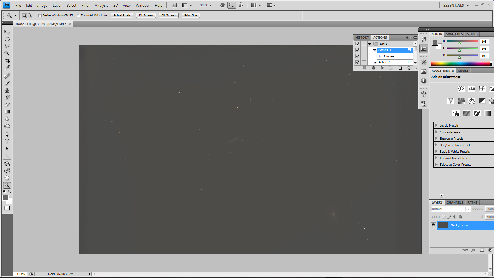 The whole frame after some initial stretching
Step2: removing the light pollution.
The image was duplicated to give a second layer and the ‘Dust and Scratches’ filter applied to it with a radius of 24 pixels. All stars disappeared leaving just the two galaxies visible. These were cloned out from adjacent parts of the image and a further Gaussian Blur applied with a radius of 24 pixels. The result is that the duplicated layer gives a very smooth representation of the light pollution which is removed from the base layer when flattening the two images using the ‘difference’ blending mode. [A very important point − reiterated below – is that though the light pollution has been totally removed, this process will also remove any parts of the image whose brightness is less than that of the pollution – in this case, the outer spiral arms of the galaxy M81.]
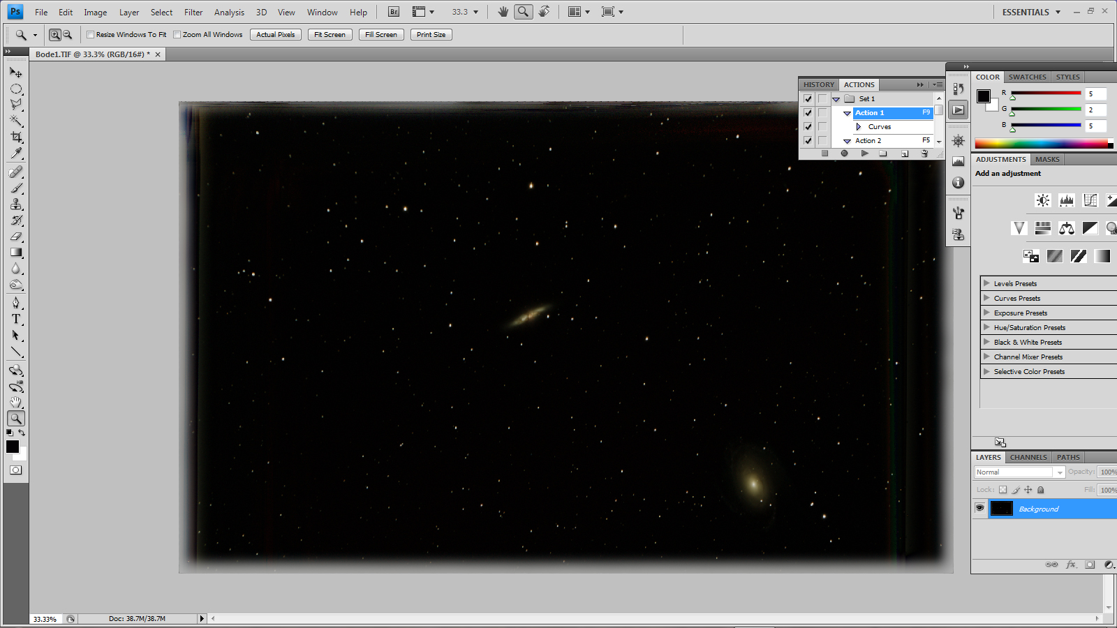
Having removed the light pollution
Step 3: further stretching.
This brings up the two galaxies and stars. The background may well be grey and this can be removed by bringing up the ‘black point’ (left hand slider in ‘levels’) a little to the right. The problem with stretching is that unless done very carefully, brighter parts of the image can become overexposed. The screen shot below shows M82 after a little stretching has been applied and, pleasingly, there is both colour and structure visible.
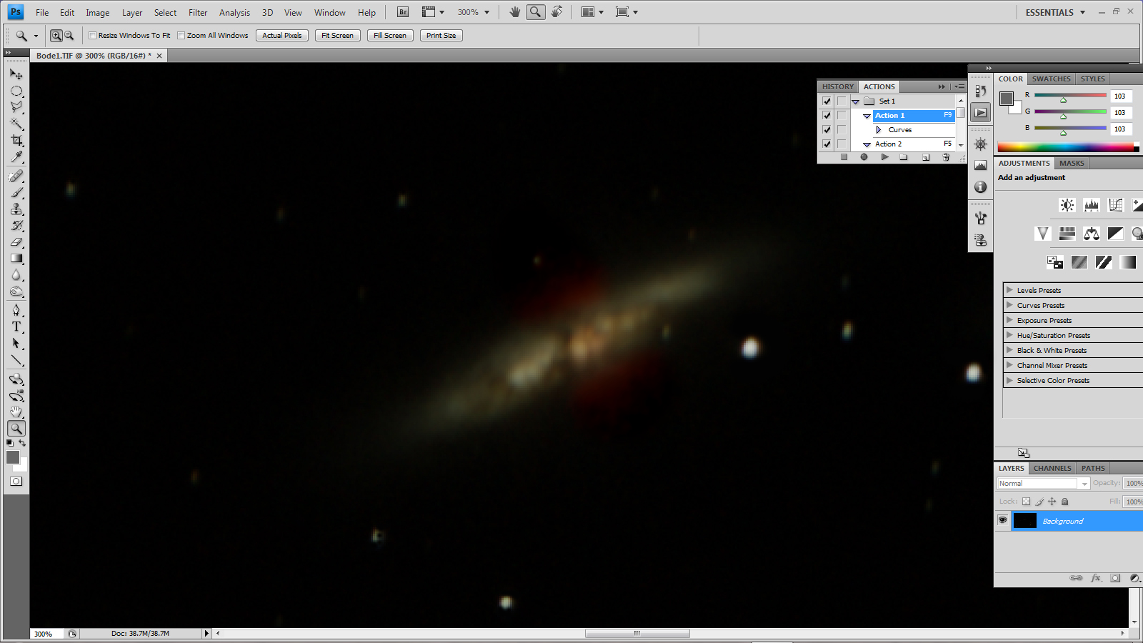
M82 after some initial stretching of the image
The object of the image is to capture, as best as possible, the two galaxies and rather than carry out further stretching of the whole image the regions surrounding the galaxies were individually selected and processed. Further simple stretching of the M82 region would bring up the outer parts of the galaxy and more of the red emission regions on either side but would burn out the central region so, to prevent this, the ‘curves’ function in Photoshop was used. The same is true for the M81 region and the screen shot below shows how some further stretching to the M81 region was applied using the this function to leave the brighter parts relatively untouched (due to the linear part of the curve) but lifting up the brightness of the fainter outer parts of the galaxy.
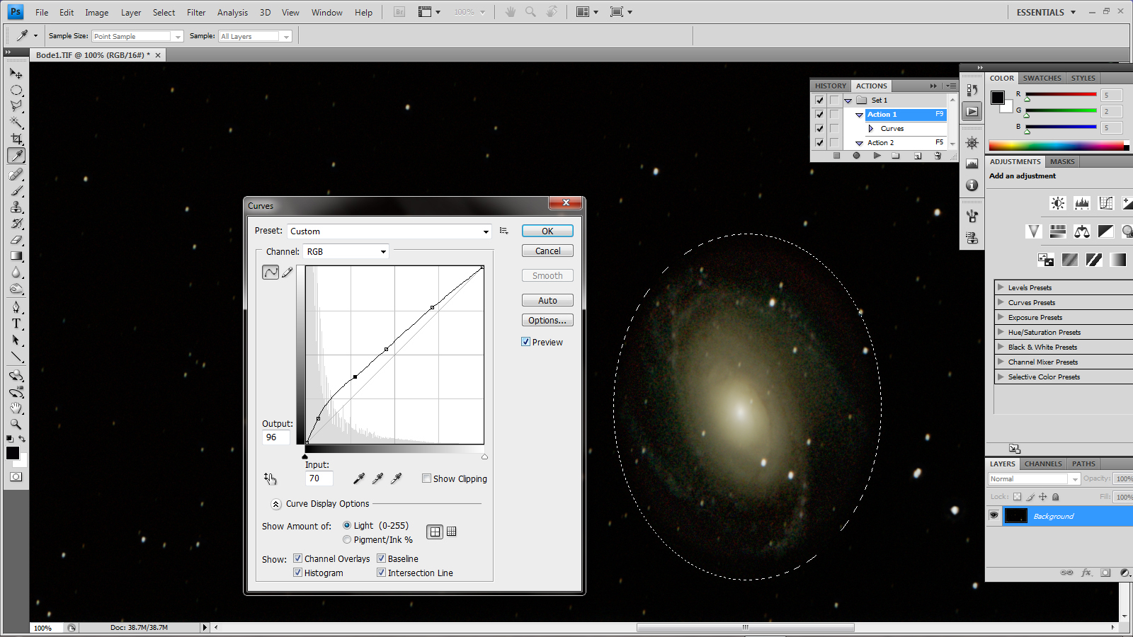 Some specific stretching of the M81 region.
Step 4: cosmetic adjustments.
A purist might state that this is all one should do, but I do think that one should be allowed to make some cosmetic adjustments to the image.
For example, the outer parts of M81 were very noisy and showed both luminance and colour noise. It seems not unreasonable to use the Gaussian Blur filter to smooth these regions to reduce both types of noise. [A Gaussian Blur can never add anything to an image!] A little de-saturation was also used to help reduce the colour noise.
I first selected the outer regions of M81.
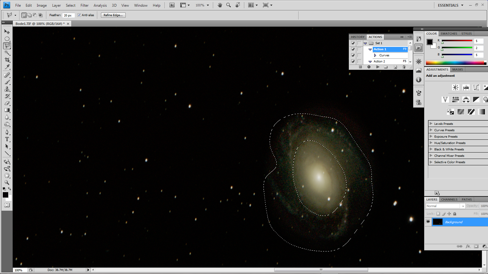
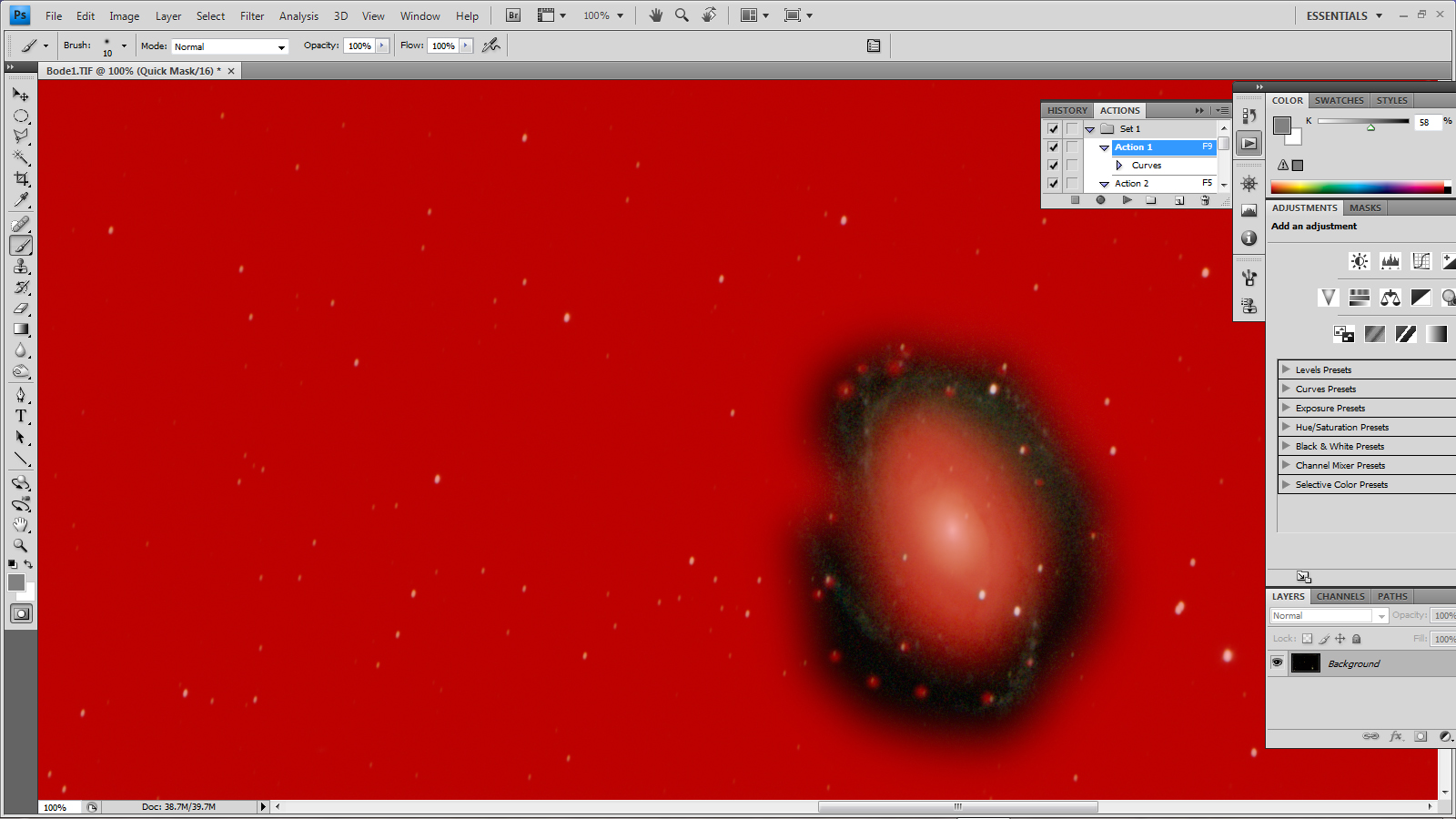
Then turned this into a mask and, using the paint brush tool, spotted out any stars within the area.
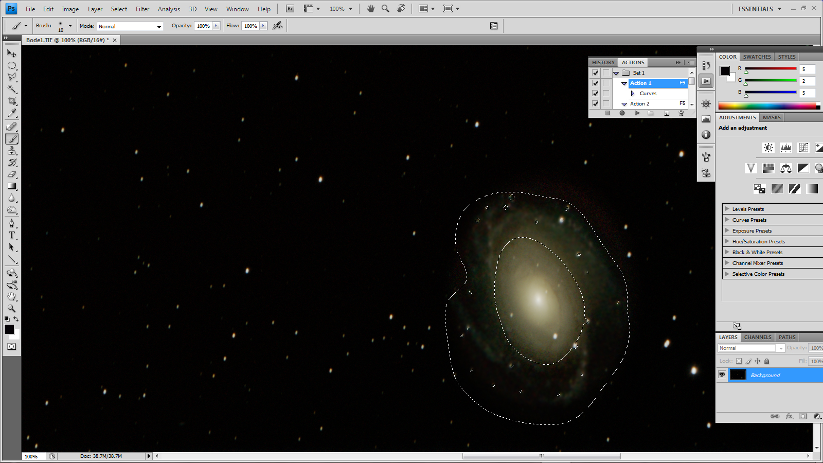
Then turned back to the ‘marching ants’ image.

I applied the Gaussian Blur with just 1.5 pixels radius which would not then be applied to the stars and a little de-saturation to help reduce the colour noise. The structure of the inner parts of the galaxy can be brought out by selecting the central regions and using the ‘unsharp mask filter’ to provide some local contrast enhancement. For this purpose, it is used with a relatively small amount, of say 15%, and large radius of perhaps 90 pixels. One adjusts these two parameters until a pleasing result is achieved.
The final image
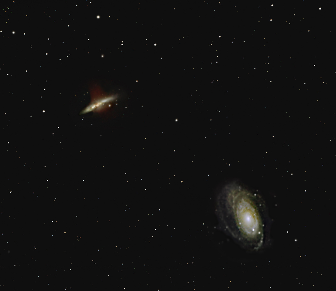
I was reasonably pleased with the final image − particularly that of M82 but not so much that of M81 whose outer spiral arms were only hinted at − though it bears no comparison with those that can be found on the web. The ideal telescope to image this pair would be an f/4 Newtonian with a Wynne corrector such as the AG8 made by Orion Optics UK. This would give a greatly reduced noise level for a given amount of imaging time. The main problem, however, was simply the light pollution from the Manchester conurbation. As shown above, it can be removed completely BUT any parts of the galaxies whose brightness was below that of the light pollution (measured in magnitudes per square arc second) will be hidden no matter how large the telescope’s aperture or the total length of exposure time. This particularly applies to the faint outer arms of M81. The night was not very transparent (I could barely see Polaris) and so a somewhat better result could be obtained on a really transparent night. However, the pair really needs to be imaged from a dark sky location!
Return to Astronomy Digest home page