Imaging the Gemini Constellation

[This is just one of many articles in the author’s Astronomy Digest.]

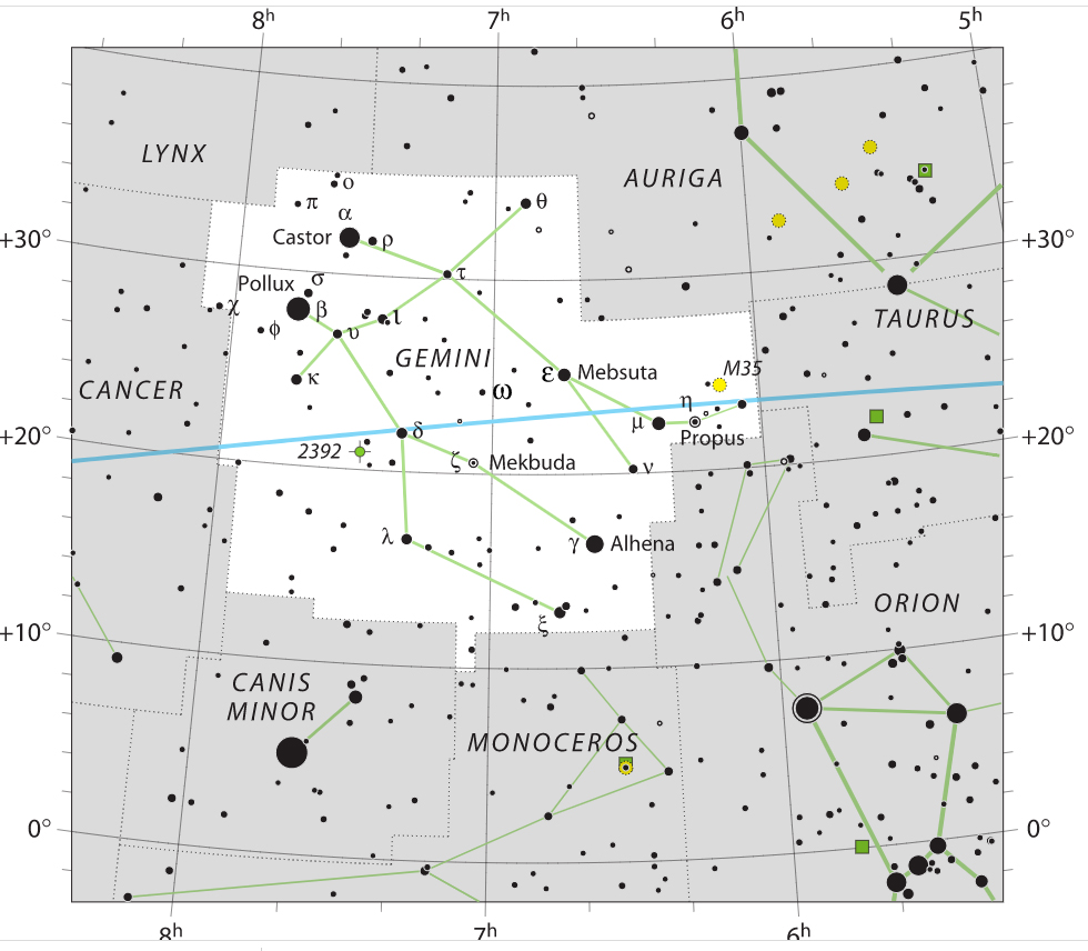
In early March, Gemini is high in the southern sky and so it is an excellent time to take a wide field image framing the constellation.   I chose to use a Sony A7S full frame camera.  It has only a 12 megapixel sensor but as the pixels, 8.4 microns in size, are quite large it has an excellent low light capability.  In fact, its extended ISO range goes up from 102,400 to 409,600!  One would never use such as ISO for imaging and, in fact, I used an ISO of 400 for this exercise.  However the camera has a most wonderful capability.  When imaging in very low light, the live view display ramps up the ISO and so stars become visible.  It is thus easy to ‘frame’ the constellation before imaging.  A second feature, now common to many cameras, is called focus peaking and, when using this, the stars become red when in focus so the camera is perfect for wide field constellation imaging.   [As I write, a ‘Like New’ A7S can be obtained from MPB for ~£654 (as mine was) with ‘Good’ ones for ~£500.]

One then has to decide on the choice of lens so that the constellation will be nicely covered.   The URL below links to a camera field of view calculator.   My best prime lens – used with an adapter on the Sony A7S – is a Zeiss 45 mm Planer.  This superb lens was designed for use with the Contax G film camera brought out in 1994 and is regarded as one of the highest resolving prime lenses ever produced.  

Using a camera Field of View calculator:

https://www.scantips.com/lights/fieldofview.html#top

gave a field of view of 43.6 x 29 degrees.  This would nicely encompass the constellation.

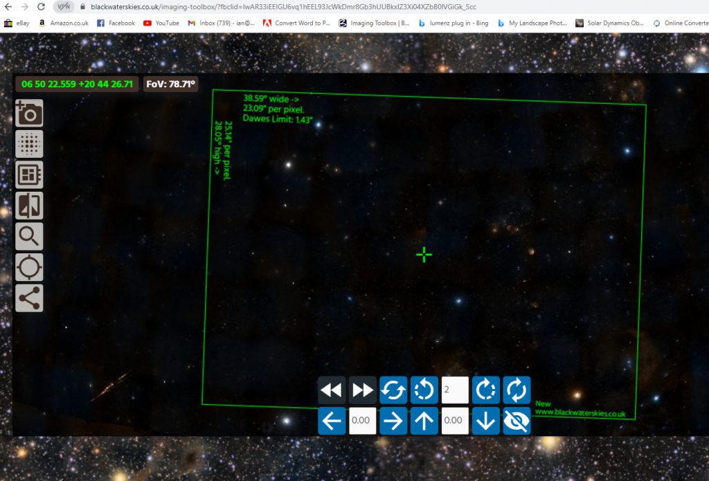
There is a very slight problem: the ‘Blackwater Skies’ field of view calculator gives a field size of 38.6 x 25.1 degrees so does not quite agree.

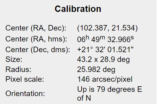
But there is an arbitrator!  As described below, the field of view was submitted to Astrometry.net to be plate solved and this was the result – Blackwater Skies is out by a little but not enough to be a real problem.

The Star Tracker

For this exercise, the camera was mounted on a rather interesting star tracker, sadly only easily available in the USA, called the  ‘The StarSync Tracker’   This is described in my digest article ‘Astrophotography Tracking Mounts’ and does not need the use of a ball head as it incorporates a camera mount capable of an even greater range of directions.  It is aligned on the North Celestial Pole using a green laser pointer laid along a machined channel and can track for up to around two hours. 

However, the alignment was deliberately made a little off as I wanted the stars to move across the sensor.  Doing so means that whilst the stars will integrate up, hot pixels will not and also what is called ‘colour mottling’ – the variation in pixel sensitivity on scales of ~ 20 pixels –  is averaged out to help give a uniform grey background.

Exposures

Using an intervalometer, I set the camera to take a series of 30 second exposures at an ISO of 400.  The lens was stopped down to f/5.6 to give its optimum resolution.  (One could easily have used longer exposures.)   A total of 153 frames were captured before clouds rolled in.  Both Jpeg and raw files were captured.  It is far easier to check though the frames using the Jpeg files to eliminate any frames where there are problems.  In this case I was able to see when the clouds came across the image and one frame showed what I suspect was a satellite spinning so that its brightness varied across the frame as seen below.

This frame could be deleted, but the trail will be removed if the ‘Sigma-Kappa’ stacking mode in Deep Sky Stacker is used as described below.  It is also well worth aligning and stacking both file types as the Jpeg files are stretched in camera and may give a more colourful image.   [It may be that the demosaicing algorithm for raw files used in Deep Sky Stacker may not be the best and an article in the digest discusses how that it can be better to use a raw converter program to first convert the raw files into Tiff files.]  As described below, there is much to be said for taking many short exposure frames rather than fewer long exposure frames.  One reason is that any star trailing will be eliminated if using a tracking mount and minimised if not when using the ‘500’ rule.  But a second reason is to do with eliminating plane and satellite trails across the image. 

Examining single 30 second Jpeg and raw exposure

It is surprising what is visible in a single exposure  (with light pollution removed) – for example the M35 cluster can be seen.  What I found pretty amazing was that no obvious hot pixels were present in this first of the frames.  But none could be seen in the last frame either – by which time the sensor must have warmed up.  This was a real surprise.

It is noticeable in the 400% crops below that the Jpeg frame is far more colourful and noisier than the raw frame.  Also, the brighter stars have an interesting pattern which is still present in the aligned and stacked final Jpeg image.  So Jpegs have introduced artefacts around the bright stars but these could easily be removed in post processing. 

Dark frames – or not

When imaging, astrophotographers are usually advised to take dark frames.  Their use will remove hot pixels and amp glow.  Using a DSLR or mirrorless camera there are two possible methods that can be employed.  The first is to use the ‘Long Exposure Noise Reduction’ mode in camera.  This follows each light frame with a dark frame and subtracts the two so removing both hot pixels and ampglow.  These dark frames will be taken at the same sensor temperature,  exposure time and IS0 and so are perfect.  The problem is that the time capturing photons is halved and a little noise will be added to the image.  [If there is a fair amount of light pollution, this will swamp the dark current noise then this will not be a problem.]   The other method is to take a set of dark frames following the sequence of light frames.  Given a long set of light frames, the sensor temperature should have stabilised and the ‘Master Dark’ frame – the average of around 10 minutes of dark frames (which reduces their inherent noise) produced when the dark frames are included in the stack should work pretty well. 

In this imaging exercise, the use of Long Exposure Noise Reduction would have reduced the signal to noise ratio by a factor of Sqrt(2) – not good.  I could have taken dark frames at the end but chose not to.  But, as I could not see any hot pixels or amp glow in the resulting image, I suspect that there would have been essentially no difference had they been employed.  [However, on a hot summer night it might well be useful to take and use dark frames.]

Aligning and Stacking the frames

Deep Sky Stacker (DSS) was used to align and stack both Jpeg and raw files.  It is interesting that the star detection threshold had to been set far lower to include sufficient stars when the raw files were processed.  This confirms that the raw to Jpeg conversion in-camera does stretch the frames to some extent.  One might think that using Jpegs only having an 8-bit depth must be worse than using raw frames having a 16-bit depth.  However if many frames are stacked when noise is present (as it will be) the effective bit depth increases so that noise (very largely light pollution) will limit the final dynamic range of the image.

DSS has a ‘Sigma-Kappa’ stacking mode.  When the image is stacked it finds the average brightness of each pixel.  It then goes through every frame and, if any pixel in a frame is too far away from the average (as produced by a plane or satellite trail), it replaces them with the average.  This does take some additional time  but removes these trails.  It may also help to remove any hot pixels.  [Without using the Sigma-Kappa method, one very low brightness satellite trail resulting from the frame shown above was visible in the stacked image.]  The result of aligning and stacking both Jpeg and raw frames were saved.

Post processing in both ‘Adobe Photoshop’ or the superb value for money program ‘Affinity Photo’

Identical steps can be carried out in both programs to process the two results:

1) The levels tools were used to move the centre slider in Photoshop or the Gamma slider in Affinity Photo to the left.  This ‘stretched’ the image and made the light pollution obvious.

2) The layer was duplicated the and the ‘Dust and Scratches’ filter applied with a radius of ~35 pixels to the top layer.  This removed the stars. 

The two layers were then flattened (Adobe) or merged down (Affinity) and the light pollution was removed from the image.

3) Some further stretching was applied.

4) The Saturation was increased.

5) A little sharpening was applied to give the final results.

Overall, the raw result was better, but the Jpeg version showed up the H-II emission nebula NGC 2174, also known as the Monkey Head Nebula, better.  I have previously found that Jpeg images are better at showing nebulosity – perhaps due to the stretch applied in the in-camera raw to Jpeg file conversion.  So I have ‘cloned’ the Jpeg version of the nebula over the raw version to give the final result as seen in the crop below.

Astrometry.net

A reduced size mono version of the image was uploaded to Astromety.net with the rather busy result below and the calibration data shown above.

Drizzling

The Airy Disk produced by the stopped down lens calculates to be ~11 arc seconds.  However each 8.4 micron pixel subtends an angle of 38 arc seconds so our image is very much under-sampled.   If the image moves across the sensor during the period of the observations then, as was used for the first Hubble Space Telescope camera which under-sampled the image produced by its 2 m mirror, it is possible to use a technique called Drizzling.  Each frame is up-sampled to 2 or 3 times its size and added to the appropriate sized grid before averaging all the frames.  Deep Sky Stacker can employ 2 or 3 times drizzle when stacking the frames and I also processed the raw data using a 3x Drizzle.

In the full sized image crop seen at the bottom of the M35 crops image, the stars are ‘smoother’.  However, if the x3 image is downsized to the same resolution as the un-drizzled image as seen in the upper two images, there is no obvious difference and the stars look very similar.  As, for web use, even this image is to be down sized, there would be no obvious gain in using drizzling unless one was wanting to make a large scale print of the constellation.

Using Images Plus to reduce the star sizes

If one has not quite nailed focus, the stars will look like round uniform brightness disks.  Though this was not the case for this image,  the free astrophotography image processing software package, Images Plus’ has a ‘Special Function’ called ‘Star Size, Halo & shape reduction’ that can be selected when an uncompressed raw image is loaded.  [Make sure Affinity Photo saves ‘Uncompressed Tiffs’.]

The lower of the comparison images below shows the result of applying the star reduction to the region around Castor and Pollux.

A real case

The upper image below shows a very small crop of an image where the focus was not perfect.  The lower shows the result of applying the star reduction tool in Images Plus four times. 

Though the stars are not perfect, when the whole image is reduced for web usage, the result is just about acceptable.