NOVEMBER 2018
Imaging the Magellanic Clouds without a tracking mount
[This is just one of many articles in the author’s Astronomy Digest.]
This article shows that it is possible to image challenging objects with just a camera and a tripod. I hope that the discussion of its production might be interesting and give an example of what is called ‘Colour Mottling’. Perhaps, surprisingly, the fact that a tracking mount was not used actually helped reduce its effects. It was carried out in October 2015 from a relatively dark location near Christchurch, in New Zealand’s South Island. The article ends with a short discussion as to the role that the Small Magellanic Cloud played in the measurement of the age of the Universe.
The main problem was that, in particular, the Large Magellanic Cloud (LMC) was not far above a light polluted horizon. Even if the light pollution is removed (as described below), no matter how long the total exposure, parts of the galaxies that are fainter than the brightness of the light pollution cannot be imaged. At the time when the individual frames were taken (using a 20 mm prime lens mounted on a Panasonic GX1 Micro 4/3 camera) I did not have a tracking mount so that the exposures were kept down to 15 seconds to eliminate star trails. [Happily, the LMC and SMC are not too far from the South Celestial Pole, so this was not too much of a problem.] This, of course, meant that, due to what is called ‘frame rotation’, the area of the sky imaged varied during the time the exposures were taken so that not all parts of the image had equal exposures. The free program Deep Sky Stacker (DSS) that was used to align and stack the individual frames can rotate the frames as well as making lateral adjustments so the majority of the final image (which included both the LMC and SMC) had the full exposure time.
Two sets of 15 second exposures were made, the first of 48 and the second of 104 frames. To reduce the effect of frame rotation the camera was realigned between the two sets. The frames were taken with an ISO of 800 (see article on choosing a suitable ISO) to give a total exposure time of 38 minutes. Each exposure was initiated manually with a delay before the shutter was released to eliminate camera shake. I would now save the frames in raw as well as Jpegs, but only Jpeg frames were taken in this case. Jpeg files have an 8-bit depth as opposed to 12-bit or 14-bit depths for raw files. However, if many 8-bit frames are stacked where there is noise in the image (as there will be) then the effective bit depth increases so little, if any, detail is lost. In addition, any Jpeg artefacts are likely to be averaged out. The good thing about having Jpeg files as well, is that they can be quickly scanned through to see if any are faulty or, if perhaps, any transient features appear. In this set of 152 frames, I first found what could well have been an iridium flare.
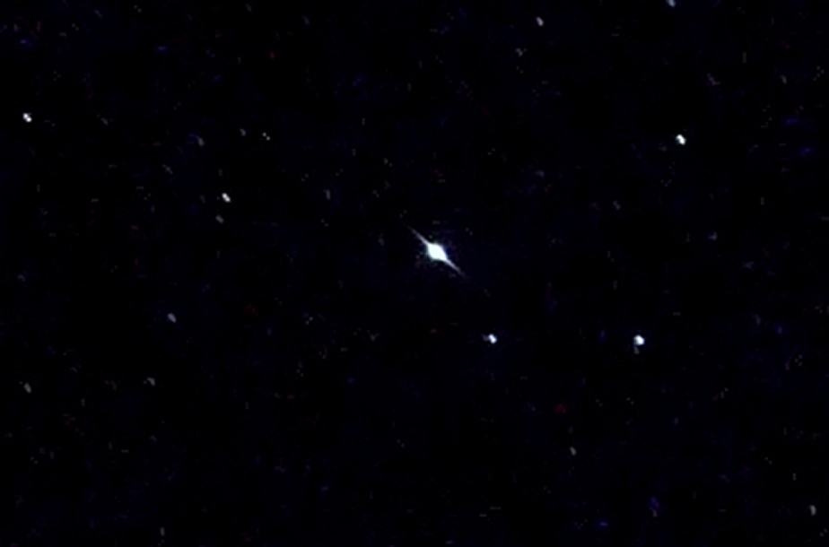 An Iridium Flare
The dark current depends on the temperature of the sensor. The heat that warms the sensor is created in the processor that produces each frame. Without a tracking mount, I was using just 15 second exposures so giving the processor considerably more work than if I had been using 60 second exposures and so, I suspect, producing more heat and thus increasing the dark current noise and making hot pixels more obvious.
Dark Frames or not?
The use of dark frames when using a DSLR or compact system camera is a rather complex subject which I have discussed in some depth in the digest article on the use of dark frames. I had chosen not to use the in-camera noise reduction but had I done so, after each 15 second light frame was taken, the camera would have taken a second exposure of the same length with the shutter closed. The good thing is that this dark frame would have been taken with the sensor at the same temperature as the adjacent light frame with the result that hot pixels would be removed from the light frame. The not so good things are that some additional noise would be added to each light frame and that the time collecting photons from the sky would be halved so requiring a longer total imaging time.
Colour Mottling
Stretching a single exposure, as seen in the crop below, does not (surprisingly) show any hot pixels but there is a mottled coloured background of largely red and blue areas. This, Tony Hallas calls Colour Mottling. [Search for ‘Tony Hallas Color Mottling’ or try https://www.youtube….h?v=PZoCJBLAYEs. (Note American spelling.)]
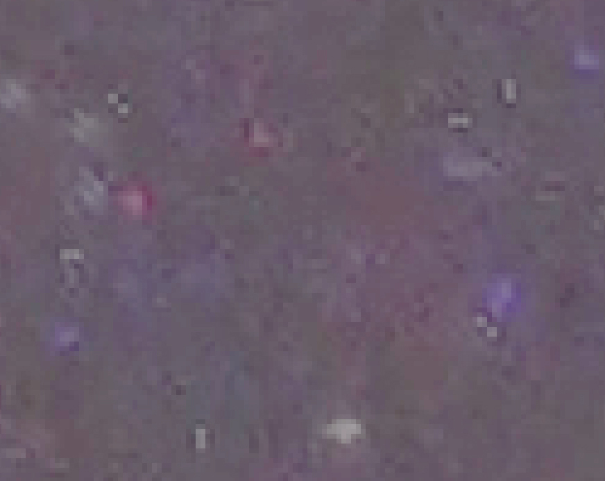 This crop shows a particularly obvious red region around 9 pixels across
The two sets of frames were stacked and aligned in DSS with the 48 frame screen shot shown below.
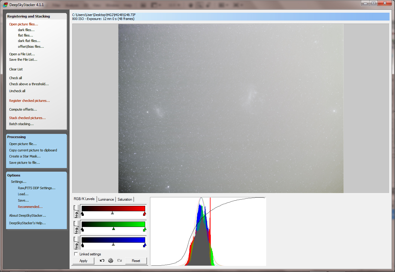
The saved image is very dark but, for some reason that I am not sure of, I applied the ‘Autocolour’ function in Adobe Photoshop and was surprised how much brighter the image appeared. The light pollution is very obvious but the effects of frame rotation less so.
Removing the light pollution
As this varies in both directions across the image, this was not too easy to remove. The objective was to produce an image in which both the stars and galaxies were removed leaving just the light pollution. The light polluted image was duplicated to give two layers and processes applied the duplicated layer. First, the ‘Dust and Scratches’ filter in Adobe Photoshop was applied with a radius of 18 pixels to remove the stars. The filter thinks the stars are dust and removes them! The two galaxies, the -0.74 magnitude star, Canopus, to the right and open cluster, NGC 2516, at top right were still visible.
These were cloned out from as close to each object as possible. Finally, a Gaussian blur of 50 pixels was applied to the whole layer to give the ‘light Pollution’ image shown below.

The layer blending mode was then set to ‘Difference’ and the two layers flattened to remove the light pollution. The result is quite dark and will need ‘stretching’ to bring out the galaxies.
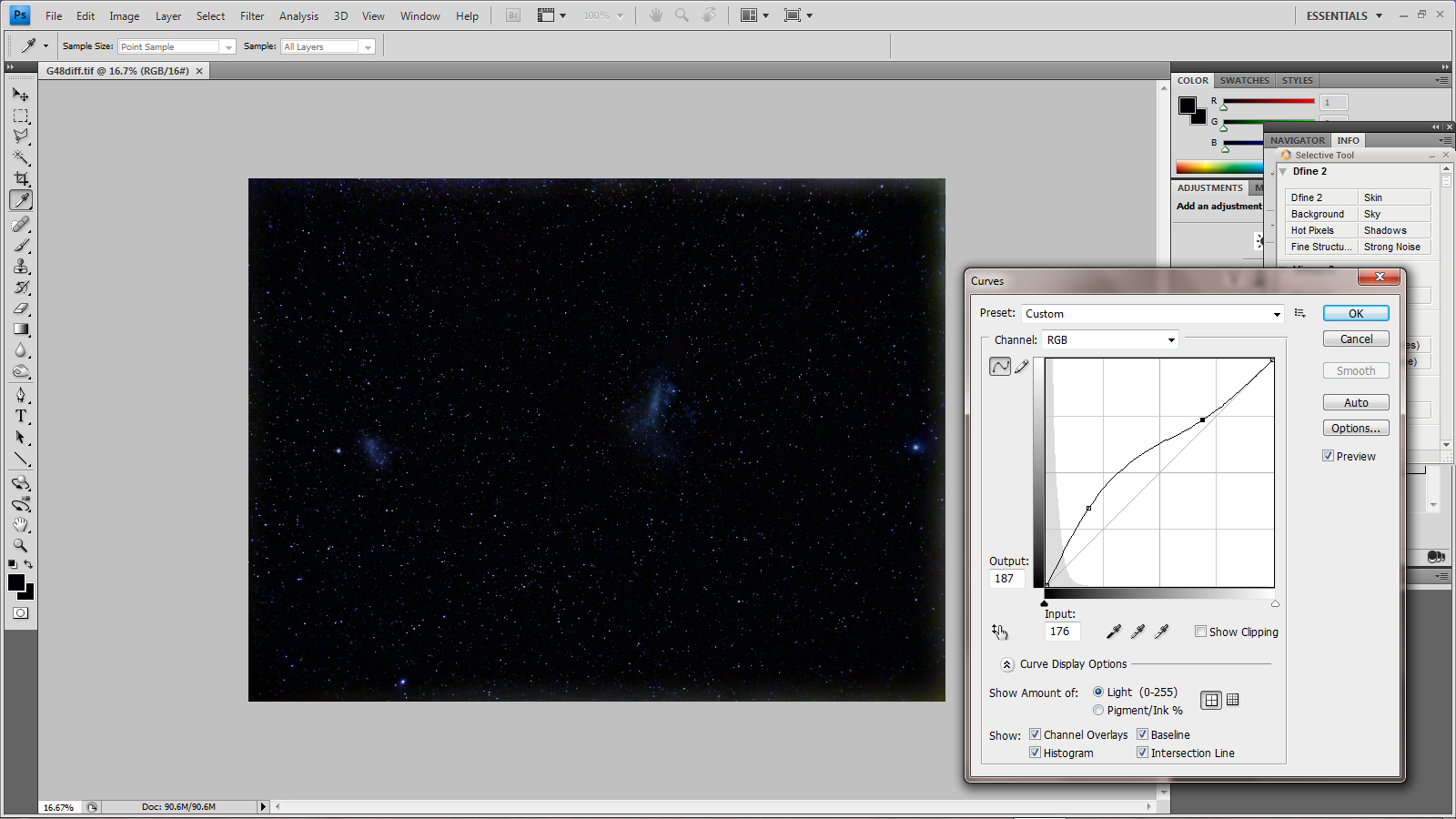
Stretching the image
There are several methods that can be used to ‘stretch’ an image such as using ‘levels’ or ‘curves’ in Adobe Photoshop or GIMP and the use of the ESA/NASA FITS Liberator program. These are discussed in some depth on the article ‘Wide Field Imaging …..’ which can be found in the digest. In this case, I found the simple use of curves gave as good a result as FITS Liberator, so used a few applications of the curve function.
Away from the stars one would hope that the sky would be a neutral grey. This is not usually the case due to changes in sensitivity of the R, G and B pixels over scales of ~10-20 pixels – the ‘Colour Mottling’ referred to above.
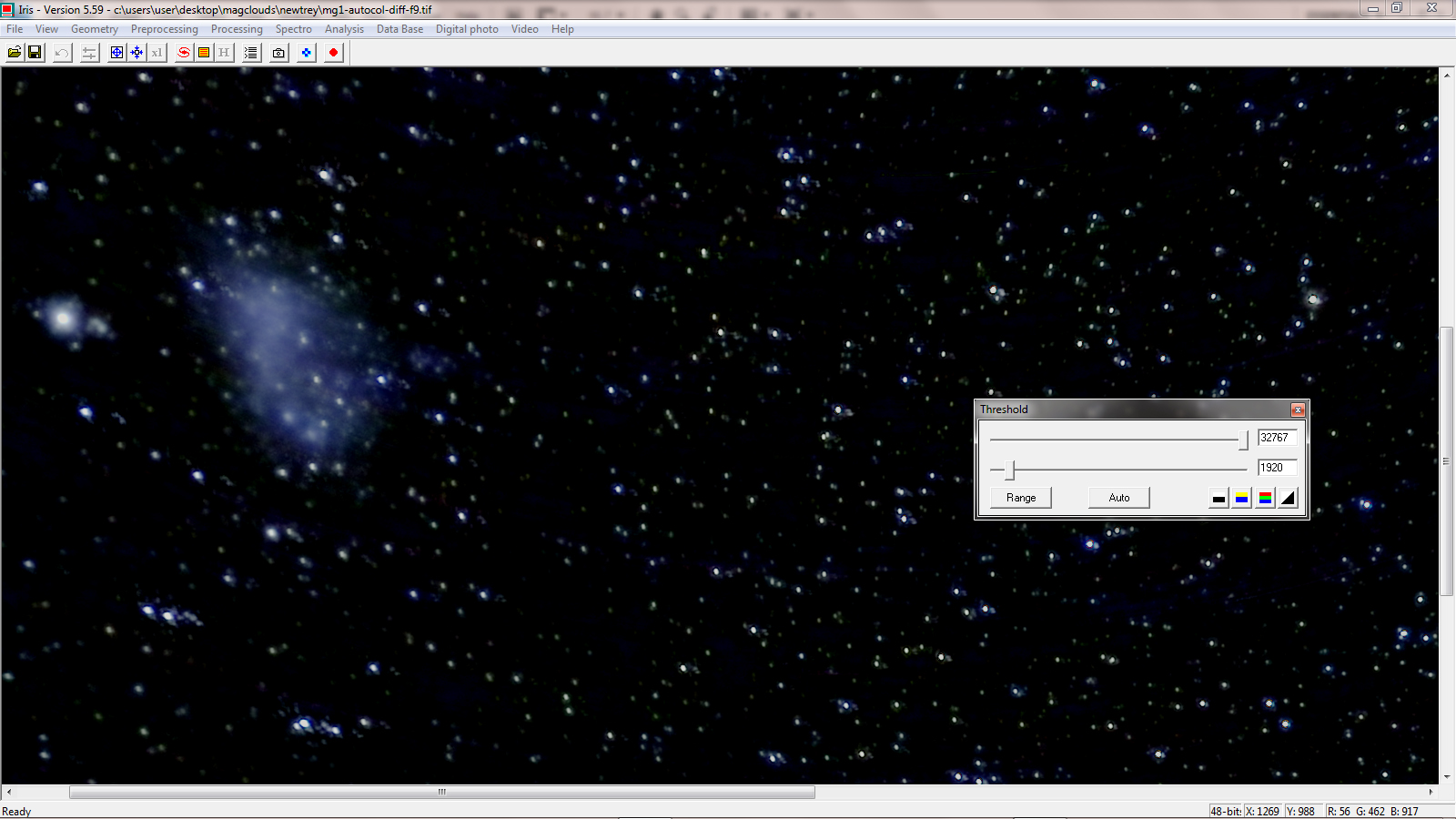
The result of moving the image over the sensor is to average the colour mottling out so making it less apparent but not totally eliminated. The effect of the frame rotation is that different coloured regions will produce a curved track in the image which will become apparent if the image is stretched too far as shown in the image below. However, this extreme amount of stretching, carried out in the free program IRIS (which can also be used to stretch an image), totally over exposed the LMC,
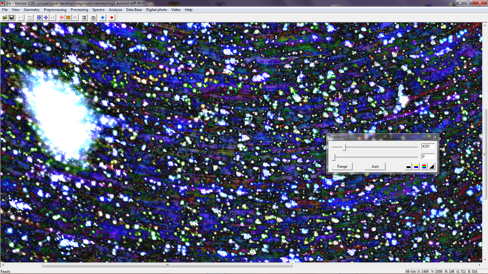 A very highly stretched crop showing the curved colour mottled regions.
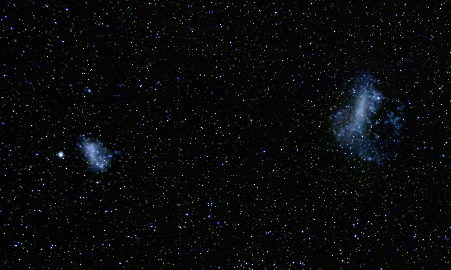
With a more suitable linear stretch in IRIS of the same region, the colour mottling has gone and the LMC is not over exposed.
 A suitable linear stretch has removed the colour mottling
[This is a very good reason for ‘dithering’ the sky image over the sensor during a set of exposures. I have my Astrotrak mounted on a Manfotto Junior Geared Head and now slightly adjust both axes at random after every ~10 frames are taken. Obviously this means that the mount does not remain perfectly aligned on the North Celestial Pole, so very long exposures are not feasible. I now believe that ~60 seconds is a good compromise to avoid star trailing with my wide angle lenses.]
Having processed both sets of frames identically, I manually aligned and combined the two images using the ‘Normal’ blending mode with the 48 frame stack given an opacity of 31%, the ratio of its number of frames to that of the total.
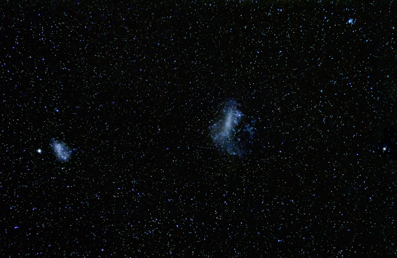
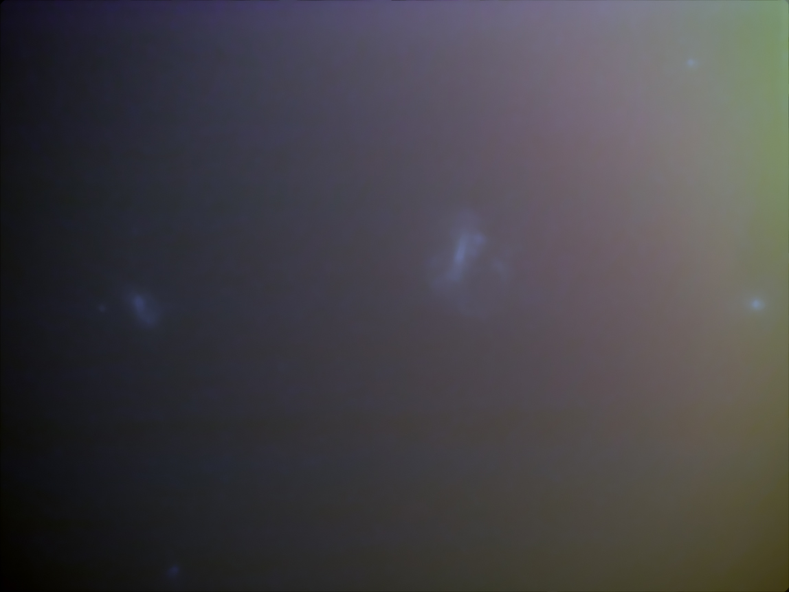
 A crop of the two galaxies
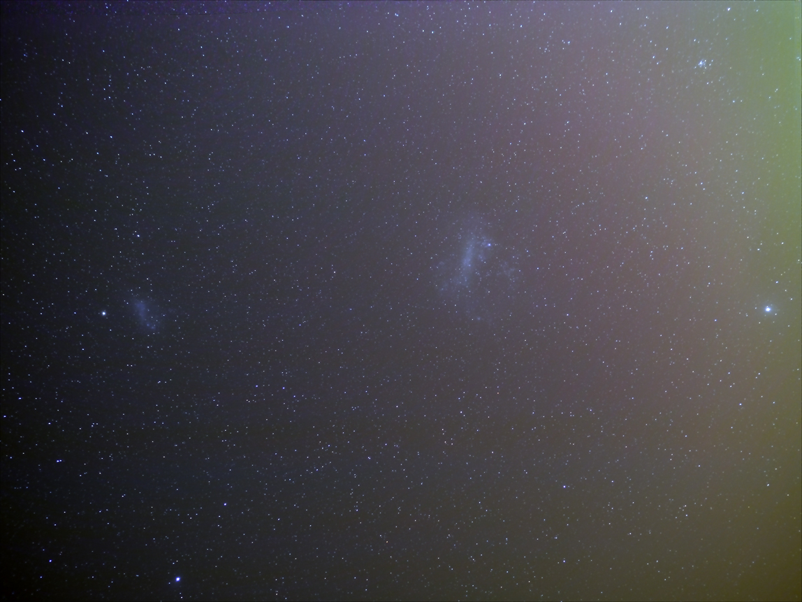
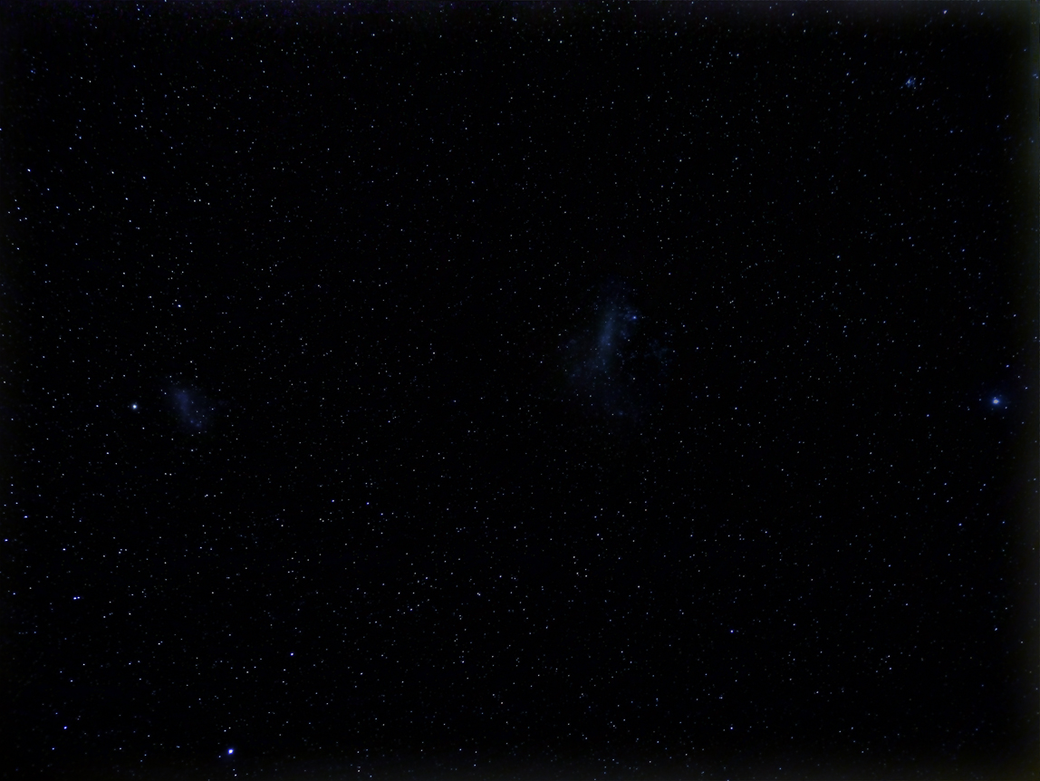
As indicated above, this is a pretty challenging region to image and really needs to be done from a totally dark location. However, some structure is seen the LMC but, as standard cameras are not very sensitive to H-alpha emission, that within the Tarantula Nebula region, does not show up. (See the image at https://www.astronomytrek.com/deep-sky-objects-small-magellanic-cloud-smc/. ) The central star cluster, NGC 2070, within the Tarantula Nebula is prominent at the top right of the galaxy and does look star-like which is perhaps the region was given the stellar name, 30 Doradus.
The LMC appears pretty amorphous but there is one interesting object over to its left. That is 47 Tucanae. If, as many now believe, Omega Centauri is regarded as the core remnant of a disrupted dwarf galaxy, then 4th magnitude 47 Tucanae is the brightest globular cluster in the heavens. It lies at a distance of ~13,000 light years and, around 130 light years across, has a magnitude of 4.1.
Canopus, or Alpha Carinae, to the right of the image is the second brightest star after Sirius in the night sky. It lies at a distance of ~310 light years and is a type A9 star having a diameter 79 times that of our Sun. There is some argument as to whether it appears as pure white or yellow-white.
The only other object of note in the image is the open cluster NGC 2516 at upper right which lies at a distance of 1.3 thousand light years. It contains a pair of 5th magnitude red giant stars and is thought to have been formed some 135 million years ago. It is sometimes called the ‘Southern Beehive’.
The role of the Magellanic Clouds in finding the distances to the galaxies
Henrietta Swan Leavitt joined the Harvard Observatory in 1903 when its director, Edward Charles Pickering, asked her to study variable stars in the Small and Large Magellanic Clouds, whose brightness had been recorded on photographic plates taken with the Bruce Astrograph of the Boyden Station of the Harvard Observatory in Arequipa, Peru. Leavitt looked carefully at the relation between the periods and the brightness of a sample of 25 of the Cepheid variables in the Small Magellanic Cloud and found that there is a simple relation between the apparent brightness of the Cepheid variables and their periods. From the known distance of the SMC she could thus find their absolute brightness and showed that, for example, a Cepheid variable with a period of 30 days was some 10,000 times brighter than our Sun.
Cepheid variable stars are some of the brightest in the Heavens and thus could be observed in more distant galaxies. Edwin Hubble, using the 100 inch Hooker Telescope at Mt Wilson observatory, discovered a Cepheid variable with a period of 31.4 days in M31, the Andromeda Galaxy, and was thus able to calculate its distance − showing that it lay far beyond our own galaxy. Later, combining his distance measurement of the 25 galaxies whose velocities of approach or recession had been measured by Vesto Slipher at the Lowell Observatory, he found a linear relationship between recession velocity and distance showing that the Universe was expanding. Projecting backwards in time until the Universe had no size he was thus able to determine its age. [NB: Vesto Slipher needs more recognition!]