[This is just one of many articles in the author’s Astronomy Digest.]

When using a webcam to image the Moon or planets, the objective is to capture as much detail as is theoretically possible given the telescope that is to be used.  There are three possible limitations that will determine the resolution that can be obtained; the telescopes theoretical resolution, atmospheric ‘seeing’ and the pixel size of the camera sensor.  If one is using ‘lucky imaging’ with a webcam and using very short exposures, one hopes that the effects of the atmosphere will be greatly reduced and then the fundamental resolution of the telescope and pixel size come into play.

As an example, this article will consider the use of a Canon 1100D camera as a webcam controlled by the excellent and free program EOS Movie Record.  To image the Moon the camera was coupled to a CFF Telescopes 127mm, f/7, refractor.  The camera is quite old and only sports a 12 megapixel sensor.  The digest includes an article ‘Using Deconvolution Sharpening with a Canon DSLR and EOS Movie Record’ related to this imaging exercise.

The resolution of the telescope is obviously the fundamental limiting factor and can be approximately derived from the simple equation: Theta (in arc seconds) is equal to 116/D where D is the diameter of the telescope aperture in mm.  So, for a 127mm refractor, this is 116/127 = 0.9 arc seconds.  (Manufacturers often quote 1 arc second for this sized aperture.)  An unobstructed aperture when imaging a star will produce an ‘Airy Disk’ of approximate Gaussian shape whose half power beamwidth will be of this size surrounded by  faint rings.  So one hopes to get as near to this resolution as possible dependant on the seeing on the night is question.

At this point, the pixel size of the camera’s sensor comes into play and what is called the ‘Nyquist sampling theorem’ becomes relevant.  This states that to extract all the information within an image, it must be sampled with a pixel size at least half that of the resolution that one hopes to achieve.   So, for this imaging example, one would ideally like each pixel to sample an area of one half of an arc second in diameter.  If the pixel size is too large, it will limit the resolution achieved.

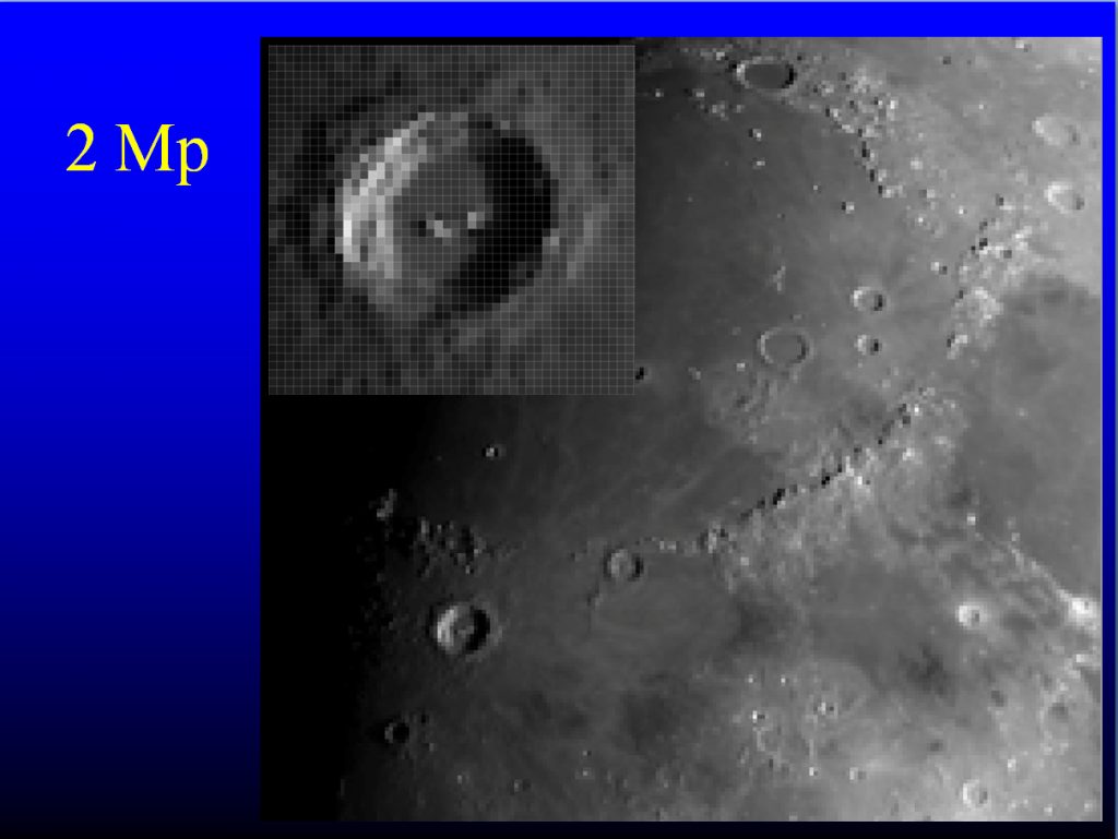
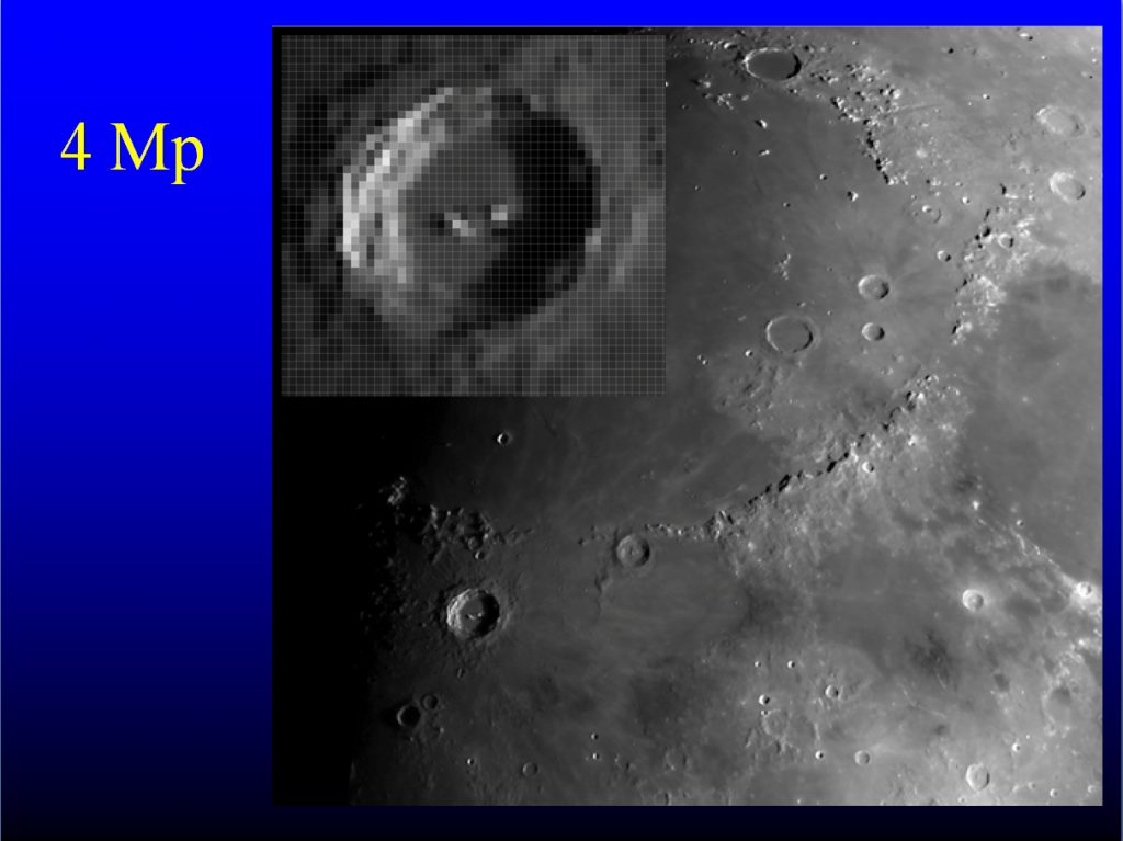
The calculation to find if this is achieved in practice will follow along with the steps that can be taken if the camera sensor has too few pixels to fully sample the image.  In order to first ‘set the scene’ is an accurate simulation of how a region of the Moon including the Appenine Mountains and the crater Copernicus would appear as the number of pixels in the sensor increases (and thus reducing  the pixel size).  The first image shows what would result if a 2 megapixel sensor were used followed by the images captured with sensors having increasingly greater number of pixels.

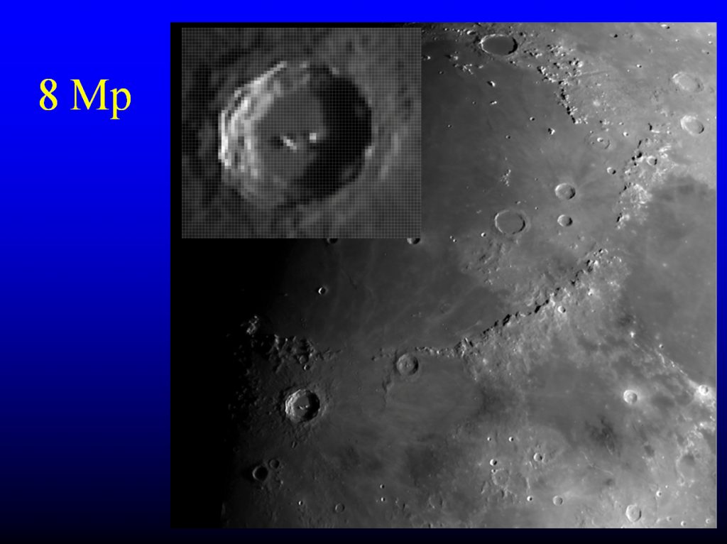
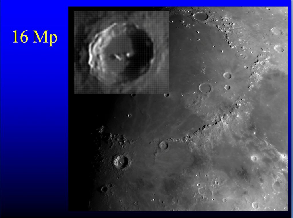
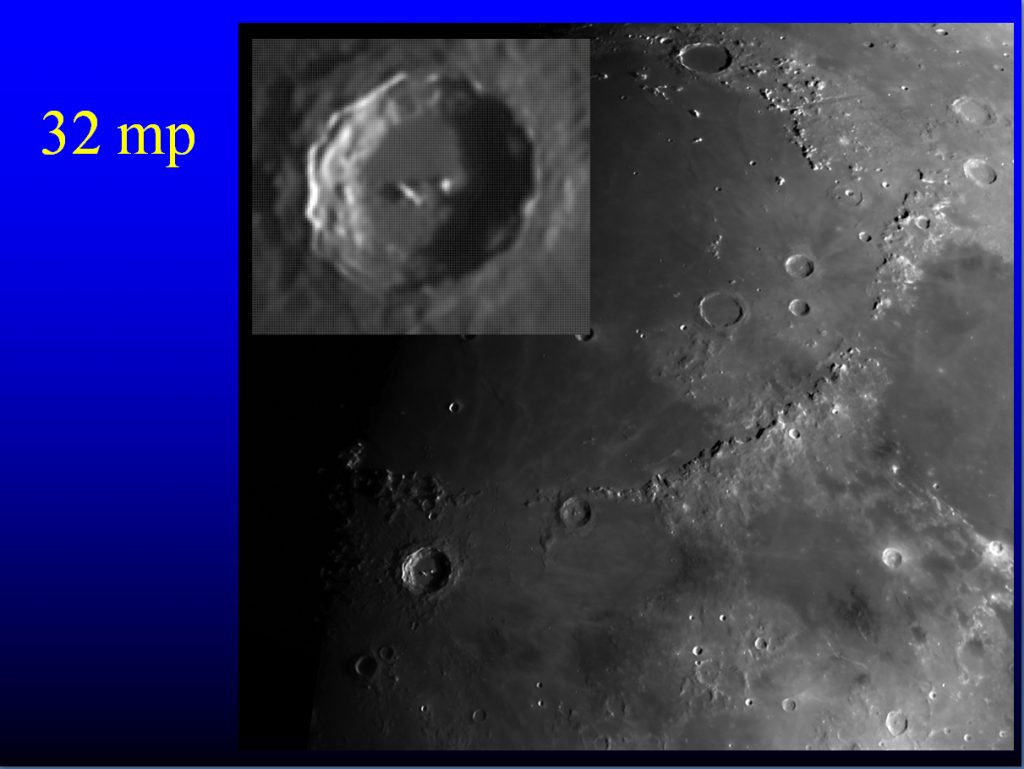
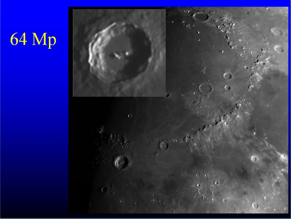
The image quality looks quite reasonable when a 16 megapixel sensor is used but, though not that obvious in the image, the 32 megapixel image is sharper.  However, the 64 megapixel image, though with smaller pixels, is no sharper; indicating that the 32 megapixel pixel size is satisfying the Nyquist sampling theorem and as much information is being captured as possible in the image falling on the sensor.  So let’s now calculate what megapixel sensor would be required and see if this matches the 32 megapixel result.

We need to first calculate the angular size of each pixel on the sensor as seen from the objective lens.  This will depend on the focal length of the telescope  ̶  the greater the focal length, the smaller the angular size that a given pixel size will subtend.  That of the CFF Telescope’s  127mm, f/7, telescope is 889 mm.  To calculate the pixel size one needs to know both the horizontal size of the sensor  – which is 22.3 mm for Canon APS-C sensors  – and the number of pixels across  – which is 6,928 for a 32 megapixel sensor.  [The 3×2 ratio sensor will have an array of 6,928 x 4,618 pixels.]  So the pixel size is  22.3/6,928 mm giving 0.00322 mm or 3.22 microns.   If this is divided by the focal length of the telescope, it gives the angular size in radians so giving 0.00322/889 radians.  To convert to arc seconds, first convert to degrees by multiplying by 57.3  and then by 3,600 to give the angular size of 0.74 in arc seconds.

One can see that, with a 32 megapixel sensor, the Nyquist theorem would just be satisfied  if the atmospheric turbulence was limiting the possible resolution to 1.5 arc seconds.  In the case of my Canon 1100D camera of only 12 megapixels, the situation is even worse with each pixel subtending  1.2 arc seconds.  It is obvious that an image taken with my camera on the 30th May 2020 would have had a lower resolution than those taken at the same time with my colleagues employing higher megapixel cameras and longer focal length telescopes.  [See below.] 

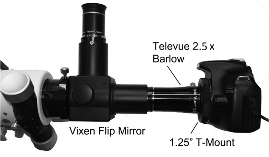
If a telescope having a longer effective focal length is used, the angular size of each pixel is reduced pro rata so, on the following night, I included a TeleVue x2.5 Barlow lens to precede the camera.  This increased the telescope’s effective focal length to 2,222 mm and hence reduces the pixel angular size to 0.48 arc seconds so complying with the basic Nyquist theorem requirement and even somewhat better if one factors in the fact that atmospheric turbulence will reduce the resolution that could be achieved.  There is, of course, a downside to this in that the area of the Moon imaged in each video sequence is reduced as so more ‘panes’ need to be used to cover the lunar surface so both more imaging and processing time is required.  (But less expensive than buying a high resolution sensor camera!)

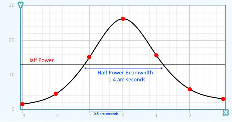
If once can find a ‘point source’ within the image, one can calculate the resolution achieved.  In the case of the images shown above, there was a mountain peak visible within the crater Copernicus which showed a Gaussian like ‘point spread function’.  This term is defined as representing what would be imaged if a bright point object were imaged.  Having measured the pixel brightness values across  the peak, a plot can be made of the ‘power’ in each pixel (amplitude squared) and the ‘half power beamwidth’ estimated as seen in the plot below.

Imaging on the night of the 30th May 2020, a colleague used an 18 megapixel Canon 700D camera coupled to a 127 mm aperture, 1,500mm focal length Maksutov.  The telescope’s resolution was thus the same as my refractor at ~1 arc second.  Each sensor pixel has a size of 0.0043 mm or 4.3 microns.  Carrying out the same calculation as described above gives an angular size per pixel of 0.6 arc seconds.  Given that the resolution that could be achieved was of order 1.4 arc seconds, his system fulfilled the Nyquist sampling theorem criteria.  It is thus not surprising that his image showed a higher resolution than mine taken at the same time using a 12 megapixel camera and shorter focal length telescope.  However, by incorporating the TeleVue x2.5 Barlow lens, the two systems became comparable and would achieve virtually identical results.