JUNE 2020
Using Deconvolution Sharpening on Lunar images captured with a Canon DSLR and EOS Movie Record
[This is just one of many articles in the author’s Astronomy Digest.]
Using the free program EOS Movie Record, one can use a Canon camera having ‘liveview’ as a Webcam to take video sequences of areas of the Moon which can then be processed in, for example, Registax 6. The advantage of this over the taking of a single image is that, by aligning and stacking the sharpest frames out of perhaps 1,000, the effects of atmospheric turbulence can be minimised so giving a sharper image. This is called ‘Lucky Imaging’.
When used to image the Moon or planets it is correct to use the x5 zoom feature. In this case, all of the pixels in the central area of the camera’s sensor will be saved in each .avi frame. As an example when using my Canon 1100D, 12 megapixel camera in x5 mode, each frame has 848x 568 pixels – exactly one fifth the size of the full frame so each single pixel is incorporated into the .avi frames. However, in x1 mode, each frame has a pixel size of 1056×704 – which means that each pixel in the .avi file is the average of 16 pixels so will not give as high resolution.
One should allow for a fair bit of overlap so that Microsoft ICE can composite the resulting ‘panes’ to give a full lunar disk. The captured .avi files are then imported into Registax 6 to be aligned and stacked. A detailed discussion of the use of Registax 6 to process lunar .avi files can be found in the article : A Lunar Imaging Example using Deconvolution sharpening and Microsoft ICE. This article also covered the use of ‘deconvolution’ sharpening which then required the use of software that was not free. Pleasingly, there is now a free software package that can be used as will be discussed below.
For these exercises, I was taking ~800 frames for each video sequence and stacking the best ~500 to give the ‘panes’ which were then composited in Microsoft ICE.
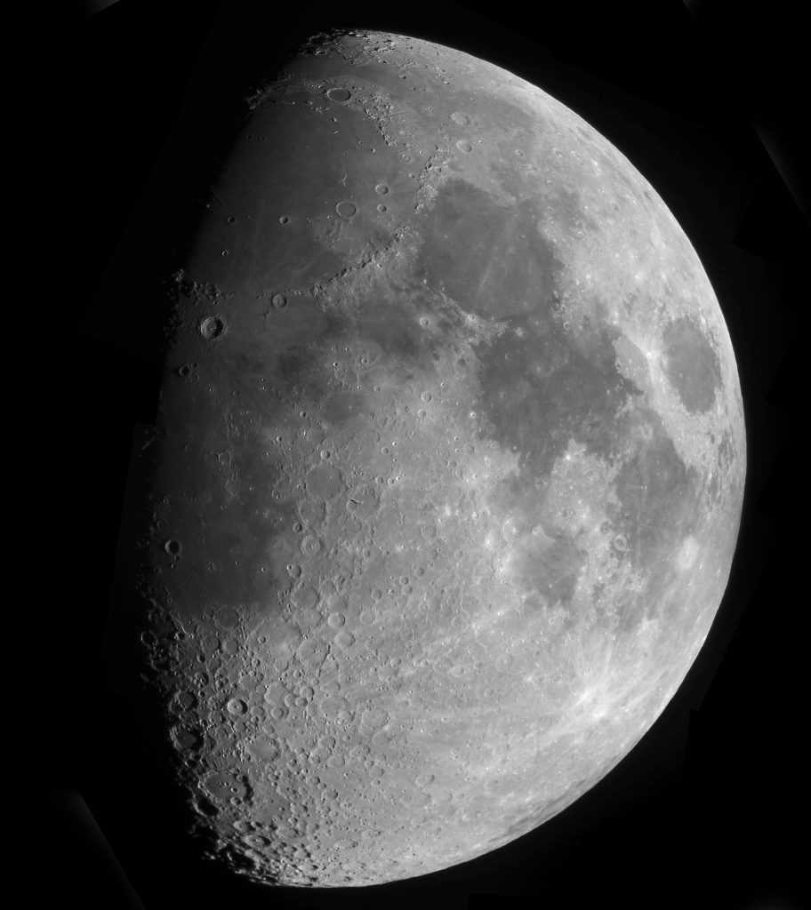
The Moon on the 29th May 2020
The camera was coupled to a 127mm, f/7, refractor and a total of 8 overlapping areas of the lunar surface were imaged. These were imported into the free program Microsoft ICE (Image Composite Editor) which then combined them to give the full disk image which was cropped and saved to be imported to Adobe Photoshop. As the Canon camera was modified to capture more of the H-alpha emission the images had an extreme red cast. A free ‘filter’ that can be downloaded from https://www.deepskycolors.com/tools.html can correct the white balance of an image if a small are of the image which should be white is first selected and then the filter applied. An alternative is to the ‘Auto colour’ tool, but this tends to overly brighten the image. A third alternative is to use the ‘Colour Balance Tool. [Quite often, a monochrome of the Moon looks best and one can simply set the ‘Mode’ to monochrome. For the first exercise I did keep the colour image as well.]
Two images were then produced with some mild local contrast and sharpening enhancements applied to as discussed in detail below: the first a monochrome image and the second with the colour saturation increased to bring out the subtle colour variations across the surface. By stacking ~500 images, a virtually noise free image results and this allows the saturation to be increased without producing ‘speckles’.
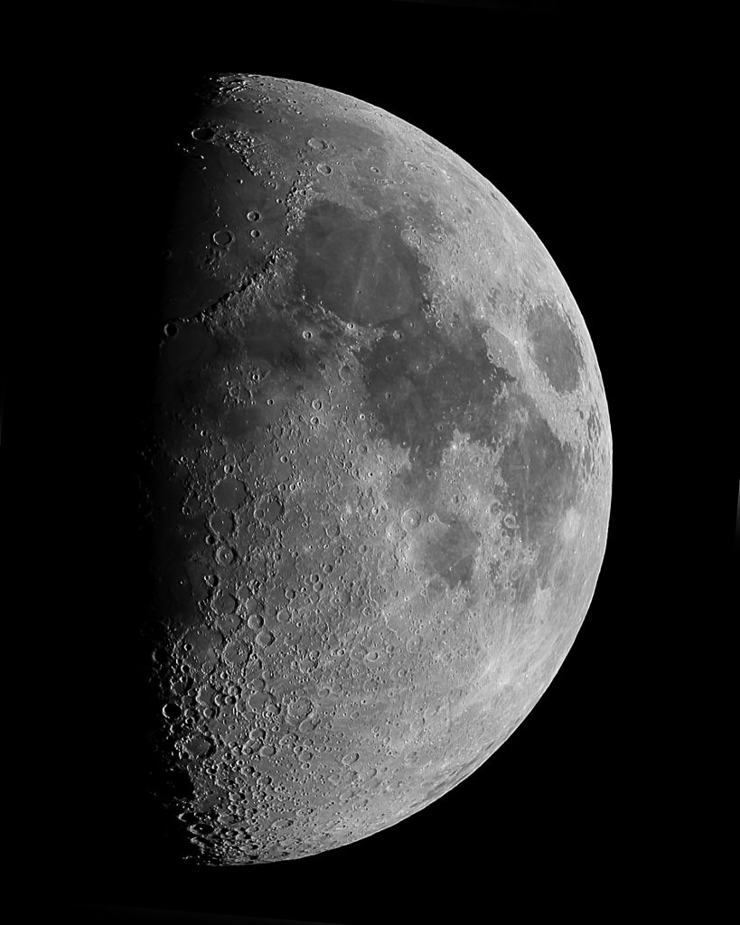
Mare Tranquillatitis is distinctly bluish in colour compared to Mare Serenatitis, above, which has a reddish colour. This is because the basalt in Mare Tranquillatitis contains more Titanium (up to 5.6% in some parts) relative to Mare Serenatitis which has a higher iron content. [I find it interesting that a remote amateur telescope can do some lunar geology!]
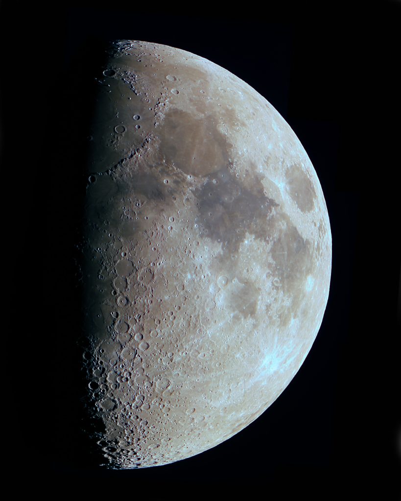
The Moon on the 30th May 2020
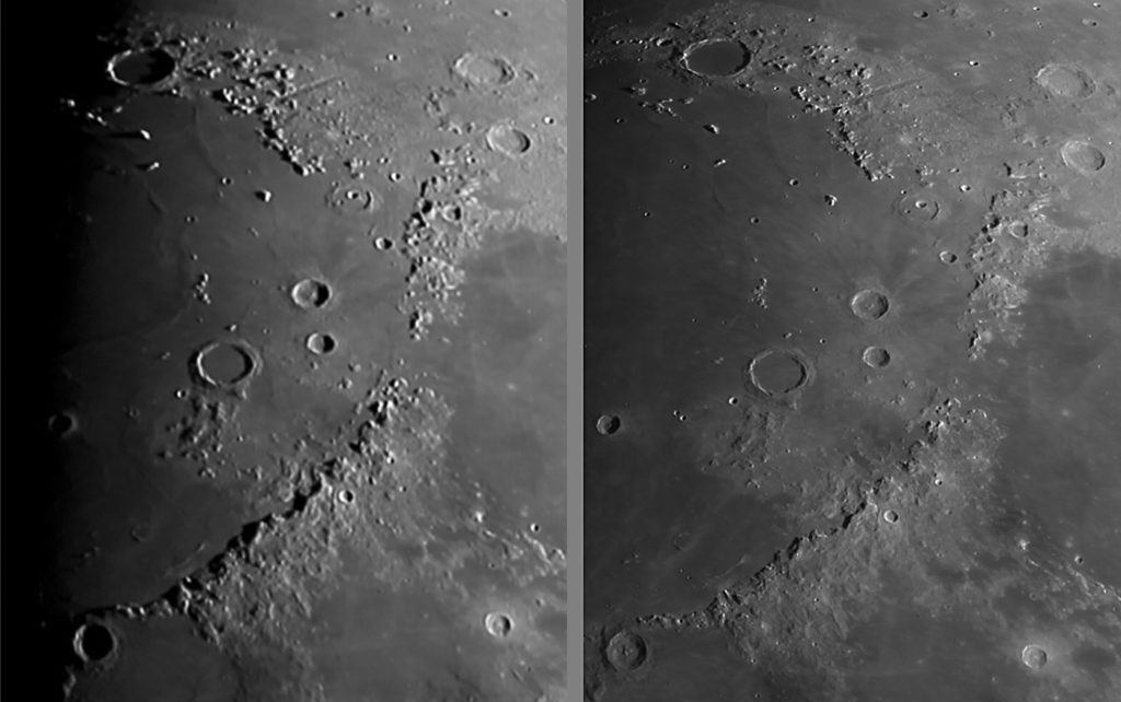
The 1100D Canon camera has only ~12 megapixels and I believe that this was the limiting factor in the resolution of the lunar image taken on the 29th May. I thus incorporated a ‘Barlow’ lens into the imaging chain, screwing the lens unit itself into the front of the T-mount tube which fits into the focuser barrel. [This gives a lower magnification that if the complete Barlow unit were used. However, the magnification that resulted was x2.2 – more than I had expected. (I was hoping for ~x1.5.) This meant, of course, that each video sequence would cover a proportionally smaller area of the lunar surface and so at least four times as many panes would be required using the x5 capture mode and so the total imaging time and processing time would be longer. However, I believe that the result was worth extra effort. The image below shows a comparison of the Appennine Mountain Range on the two nights. Though the lunar phase had changed and thus this is not a perfect comparison I think that it is obvious that the resolution had increased.
Enhancing the lunar image
The lunar images taken on both nights can be enhanced; by first applying some local contrast enhancement and then by applying some sharpening.
Localcontrast enhancement
A simple way to do this is to use the ‘Unsharp Mask’ filter with alarge radius and relatively small amount. (The opposite to when it used tosharpen.) This tends to darken the Mareregions relative to the highland regions. However it can over-brighten the bright limb regions so I usuallyselects this region with a fairly wide feather and then invert the selectionbefore applying the filter. Some trialadjustments will enable a good balance to be achieved.
Sharpeningthe image
There are many methods of sharpening; some of which are beautifully described in an Affinity Photo Video – search for ‘Affinity Photo Sharpen five ways’. These can be also employed in Adobe Photoshop. They include ‘Unsharp Mask’, ‘Smart Sharpen’ and ‘High Pass Sharpening. Though ‘Smart Sharpen’ may be a little more sophisticated, these effectively add ‘acutance’ to an image by increasing the ‘microcontrast’ at changes in brightness in the image: if at an edge in an image the brightness went from a dark grey to a light grey, at the dark grey side it would be made darker and at the light grey side it would be made lighter so accentuating the difference. The image below, at ~400%, shows precisely this . Smart Sharpen was applied to the brightness change in the top image to give the result below. [Pleasingly this worked exactly as I had expected.] There is also the problem of the bright ‘halos’ that these methods can produce. I do not believe that these methods actually sharpen an image, they only appear to make them sharper. (This may be pedantic.)

High Passsharpening
This is rather similar process to the above but takes a littlemore effort. The image is duplicated andthe ‘High Pass’ filter applied to the duplicate layer with a radius of a fewpixels. This layer becomes mid greyexcept at the edges within the image. The blending mode is set to ‘Overlay’ and the sharpening amount can becontrolled with the opacity slider. Anice ‘sharpening’ tool.
Waveletsharpening
This is a very interesting method of sharpening and is available in Registax 6. The image is dissected into 6 layers each containing information in differing ‘spatial frequency’ bands – from large scale features to very fine detail. The brightness of each of these layers can be individually adjusted and if, in particular, the brightness of the three finest layers (1 – 3 in Registax) is increased, the sharpness of the image will be enhanced. This is very probably a better method than the ‘acutance’ methods above, but again I am not sure that this is true sharpening. I say this because there is a method that really does attempt to increase the sharpness of an image as discussed below.
DeconvolutionSharpening
Deconvolution Sharpening was developed to improve the images fromthe Hubble Space telescope before corrective optics were added to compensatefor its improperly shaped mirror. It isalso said to be used to enhance the images from spy satellites!
Let me try to explain, but skip this bit if you like. Let’s assume that one is using a 127mm aperture telescope to image the Moon and there is no atmospheric turbulence (we wish). The image that would be captured would be the actual image ‘convolved’ with the diffraction effect of the limited aperture – an Airy pattern with a central disc of around 1.2 arc seconds in size surrounded by lower brightness rings. The central disk would have an approximate Gaussian shape. If the deconvolution sharpening software ‘knows’ the shape of this ‘point spread function’ (as this is what would be seen if a point source were imaged) then the software attempts to deduce what the original would be like. Usually a Gaussian point spread function is used – which approximates well to the central Airy disk when a telescope is used. One can define its size which depends on the image scale of the pixels used to capture the image. (As an example, the pixel image scale used when the May 31st image was produced was 0.5 arc seconds so, given a resolution of the telescope of just over 1 arc second, a 3×3 size Gaussian point spread function was appropriate.
Softwareto implement deconvolution sharpening
For some years I have been using the excellent program Astra Image to sharpen my lunar images, but there are now a couple of free alternatives.
The first is found in the, now free, astroimaging package Image Plus. Having opened up the ‘Smooth Sharpen’ menu, the tool ‘Adaptive Richardson – Lucy Restoration’ isselected. This brings up a controlwindow. The initial default settingswork well but one can alter both the ‘Point Spread Function’ size and thenumber of iterations applied. I doselect the ‘Reduce Artifacts’ box. Againtrial applications are needed to give the best result.
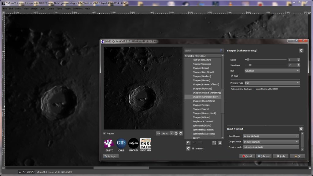
There is now, I feel, a better alternative available within the free program GIMP once a set of filters has been downloaded from gmic.eu/download.shtml. This collection of filters is free but a contribution would be appreciated. It has an excellent control window which, like Astra Image, allows one to immediately see the effect on a small region of the lunar surface as the sharpening parameters are changed before then committing to the overall result.
Having installed the GMIC filters, at the bottom of the GIMP included filters should be seen ‘G’MIC-Qt..’. Clicking on this brings up a window with a list of the filters at its right. The magnification should be adjusted so that an interesting region of the lunar surface is seen well as in the screenshot below – I selected the crater Copernicus. The ‘Details’ sub menu should be opened up and the ‘Sharpen [Richardson-Lucy]’ filter should be selected when the appropriate control sliders appear to the right.
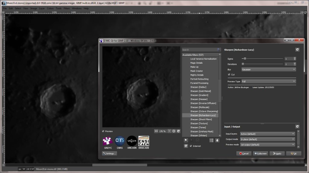
I suggest leaving the Sigma value at 1 and certainly use ‘Gaussian’ for the point spread function. By adjusting the number of iterations to be applied, the sharpened result can be immediately seen. For this image, I felt that 12 iterations was about right. When satisfied the OK button is clicked upon and then the devolution iterations are applied to the whole image, taking some time. When finished, the sharpened image appears in the main GIMP screen and is saved (actually ‘exported’ in GIMP).
Though the image is truely sharpened, it may well not look as sharp as if the actuance type ‘sharpening’ filters have been used and it may be worth applying some additional ‘sharpening’ either with ‘Smart Sharpen’ or, as I used, ‘High Pass Sharpening’ with a radius of 3 pixels the opacity reduced to ~50%. But I did notice that in some crater walls the resolution was actually reduced a little!
There is one thing that I do not fully understand. All three of the GIMP, Image Plus and Astra Image programs take some considerable time to carry out the number of iterations selected – it is an iterative process which is computationally intensive – whereas some filters that claim to carry out deconvolution sharpening are virtually instantaneous. There is something not quite right here.
The results
First the full image at reduced resolution followed by larger scale areas of the surface.
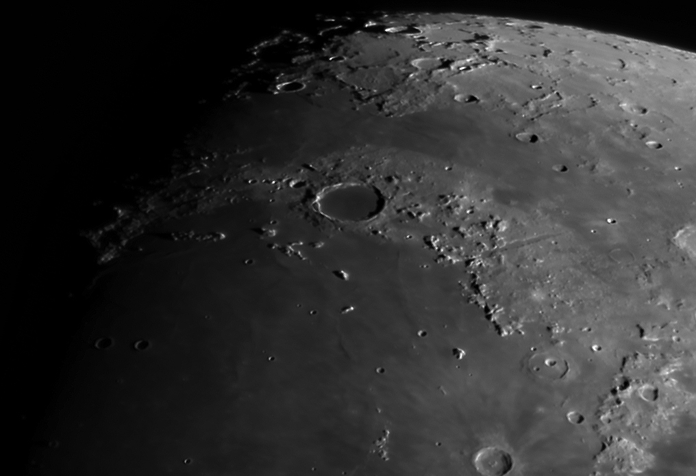
Plato and the Alpine Valley
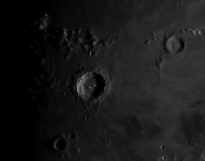
Copernicus
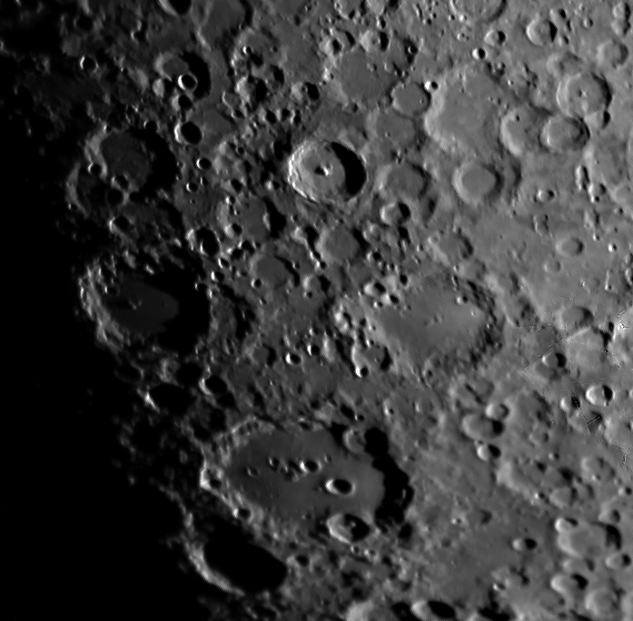
Plato and Clavius
This is my second best image of the Moon following that shown in the Lunar section of my ‘Night Sky’ page (search Night Sky Jodrell) which was, however, imaged using a 200 mm aperture telescope and Point Grey Chameleon webcam in the infrared.
Thoughtsabout resolution
The full lunar image taken on the 30th May was 3,600 pixels in height. As the Moon is ~30×60 arcs seconds across (so ~1,800 arc seconds), this meant that each pixel was subtending 0.5 arc seconds. This would just obey the Nyquist sampling theorem if one were hoping for a resolution of 1 arc second. In fact one could not really expect a lunar image to have this resolution when a 127mm refractor were used also making an allowance for the atmosphere. I thought that this image would have achieved a resolution of between 1.25 and 1.5 arc seconds which is really quite creditable and this was proven as seen below. [As mentioned above, using a 200mm aperture telescope and imaging in the infrared where the atmosphere has less effect, I have achieved ~0.7 arc seconds.]
It is actually possible to estimate the resolution achieved by finding as close to a bright point in the image as possible. In this case a mountain top within the crater Copernicus provided an excellent ‘point source’.
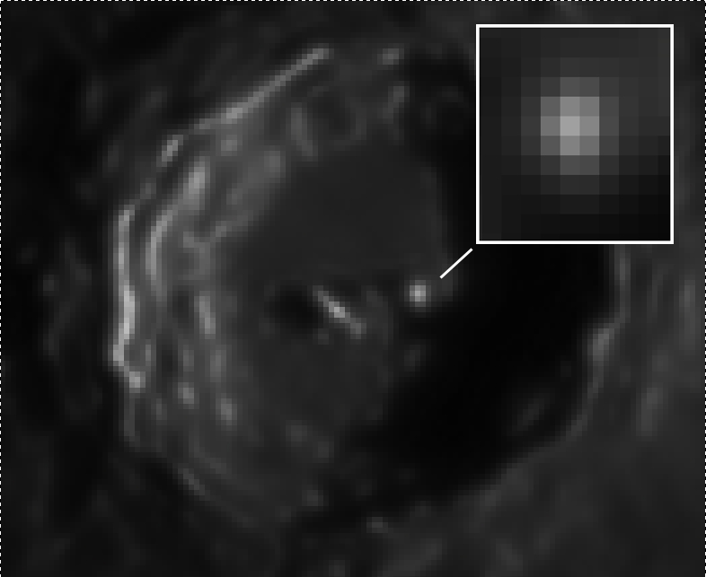
Using the ‘Info’ tool one can measure the brightness of pixels across the peak and this gave the values: 39, 67, 123, 162, 125, 72, 55. These are amplitudes so the ‘power’ values would be the square of these (scaled down): 1.5, 4.5, 15.1, 26.2, 15.6, 5.8, 3.0. Using the MyCurveFit plotting software, this produced the following plot.
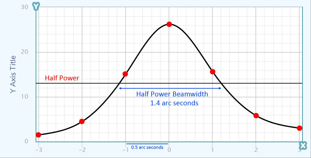
This gave a half power beamwidth of 1.4 arc seconds. As the target ‘point source’ is unlikely tobe an actual point source, the achieved resolution could be somewhat less thanthis. A very pleasing result.
This is just one of over 100 articles in the author’s Astronomy Digest.